Read · Brownian motion · Explanation preview

§4 · From random displacement to diffusion

Detail

Letters

Show modern qualifications

Einstein's letters change 1 of this paper's 18 formulas. 1 is already in his letters, and 16 stay in today's letters, with a note saying so.

JavaScript is off. The full explanation is shown. Each passage’s “Show every step here” disclosure works without scripts, and foundation links open complete reading pages. The embedded laboratory remains a static worked example.

First encounter · No algebra required

Do particles that wander in all directions ever get anywhere?

Imagine placing a microscopic particle in a drop of water and marking where it is after a few moments. Pushed at random by invisible water molecules, it is just as likely to move left as right. In the symmetric arithmetic example below, signed displacements cancel even though all four endpoints differ from the starting point.

Authored arithmetic examples: Displacements of −3, −1, +1, and +3 units (three steps left, one left, one right, three right). These are an authored educational case, not a measured dataset.

Step 1 · Explore the particle displacements

Drag a marker or select it and use ← / → arrow keys to shift its position.

Particle 1-3 units(three steps left)

Particle 2-1 units(one step left)

Particle 3+1 units(one step right)

Particle 4+3 units(three steps right)

Signed total0 unitsMean: 0.0 units

Mean distance, ignoring sign2.00 unitsProposal A (ignore sign)

Mean square5.00 squared unitsProposal B (square first)

Root mean square (RMS)2.236 units√(mean square)

Steps 2 and 3 · What a signed sum tells us

When we add the displacements algebraically, opposite directions cancel out:

(−3) + (−1) + (+1) + (+3) = 0 units

A signed total of zero tells us that the average endpoint has not shifted. It does not mean every particle remained at rest. In the authored example all four particles have nonzero displacements; after your edits the displayed totals describe your chosen endpoints.

Steps 4 and 5 · Two ways to keep track of distance

How do we keep track of how far particles wandered without opposite directions cancelling out? Both of these proposals are reasonable:

Proposal A (ignore the direction): Take the absolute value of each displacement. For our authored example (−3, −1, +1, +3), the absolute values are 3, 1, 1, 3 units, giving a mean absolute displacement of 2 units.
Proposal B (square each displacement): Multiplying any negative number by itself produces a positive number. The squared displacements are 9, 1, 1, 9 squared units, giving a mean square displacement of 5 squared units (and an RMS distance of √5 ≈ 2.236 units).

Steps 6 and 7 · What happens when every displacement doubles?

Suppose after a longer interval every particle has wandered twice as far (−6, −2, +2, +6 units):

Mean absolute displacement:(|−6| + |−2| + |+2| + |+6|) / 4 = 4 units (doubles from 2)

Mean square displacement:(36 + 4 + 4 + 36) / 4 = 20 squared units (quadruples from 5)

Notice that when displacement distances double, the mean square quadruples (2² = 4 times larger), and its square root (RMS = √20 ≈ 4.472 units) doubles exactly in proportion to distance.

Step 8 · Why the mean square has a simple additive rule

Both proposals measure spread. The mean square has a useful property when independent, zero-mean displacements are added. This is a pedagogical bridge, not the paper’s printed calculation.

First expand the square of a sum. This algebra holds without an independence assumption:

(Δx₁ + Δx₂)² = Δx₁² + 2 Δx₁ Δx₂ + Δx₂²

Now assume the displacements over the chosen time intervals are independent and each has zero mean. Independence makes the average product equal the product of the averages, so the cross term vanishes on averaging, not in every outcome. Equal finite step mean squares then add in proportion to the number of intervals. This coarse-grained assumption is not a claim about molecular motion at arbitrarily short times.

Absolute values have no such rule: the average absolute value of a sum is not, in general, the sum of the average absolute values. That is why the mean square is the measure that adds.

Step 9 · Mean absolute displacement is not a wrong answer

It measures spread too: the average distance from the start, ignoring direction. For the ideal Gaussian spread it also grows with the square root of time; along one coordinate it equals √(4Dt/π). The mean square is the one the argument uses because of what step 8 showed: for independent steps, mean squares add.

Why the square is useful: two steps, worked out

Take two successive independent steps, Δx₁ and Δx₂, each equally likely to be +1 or −1. The four possibilities are equally likely:

+1 then +1: total +2, squared 4
+1 then −1: total 0, squared 0
−1 then +1: total 0, squared 0
−1 then −1: total −2, squared 4

The average total is (2 + 0 + 0 − 2) / 4 = 0. The average square is (4 + 0 + 0 + 4) / 4 = 2, which is 1² + 1²: the squares of the two steps add. The cross terms, 2 Δx₁ Δx₂, are +2, −2, −2 and +2, and they average to zero.

Why do the cross terms vanish? Open the exact missing step

Static reference (JavaScript disabled)

With JavaScript disabled, the complete worked arithmetic is presented statically below:

Authored example (−3, −1, +1, +3 units):
Signed sum = (−3) + (−1) + (+1) + (+3) = 0 units.
Mean absolute displacement = (3 + 1 + 1 + 3) / 4 = 2 units.
Mean square displacement = (9 + 1 + 1 + 9) / 4 = 5 squared units.
Root-mean-square displacement (RMS) = √5 ≈ 2.236 units.

Doubled example (−6, −2, +2, +6 units):
Signed sum = (−6) + (−2) + (+2) + (+6) = 0 units.
Mean absolute displacement = (6 + 2 + 2 + 6) / 4 = 4 units.
Mean square displacement = (36 + 4 + 4 + 36) / 4 = 20 squared units.
Root-mean-square displacement (RMS) = √20 ≈ 4.472 units.

Open the foundation on mean, variance and RMS Open the tracer-ensemble laboratory Go to the §5 displacement passage

A definition

Zero average is not no movement

What can we measure when left and right cancel?

The 2 printed paragraphs this passage explains

§4, paragraph 9: The displacements in any time t are distributed like random errors; what matters is how the constant in the exponent depends on D, and it gives the root of the mean square displacement along X, λx, as the square root of 2Dt.
§4, paragraph 10: The mean displacement therefore grows as the square root of the time, and the root mean square of the total displacement in space is λx times the square root of 3.

A signed mean answers where the ensemble’s centre has moved. It does not answer how far its members have wandered. For a centred distribution, rightward and leftward contributions balance even while the distribution broadens.

\langle x\rangle=0,\qquad\langle x^2\rangle>0

The model’s mean displacement can be zero while its mean-square displacement is positive.

To retain the movement, square each displacement before averaging. Taking the square root of that mean square returns a length: the root-mean-square displacement, or RMS. A mean absolute displacement is a different observable, and neither is the length of a wandering trajectory.

Open the foundation: Mean, variance and RMS

Show every step here: Zero average is not no movement

A tool for this step

Adding and averaging

What does an average keep, and what does it lose?

Four jars hold 3, 1, 1 and 3 marbles. Pour them together and there are 8. Share the 8 equally between the four jars and each holds 2. Two is the average, although no jar held 2 to begin with.

The average keeps the total and the count and nothing else, so 3, 1, 1, 3 and 2, 2, 2, 2 have the same average. Listing every value twice doubles both the total and the count, and the average stays at 2.

Worked example: Three mornings with the same average

One morning the four jars hold 3, 1, 1 and 3 marbles. Add them: 8. Divide by the four jars: an average of 2.
Another morning they hold 8, 0, 0 and 0. Add them: 8 again. Divide by four: 2 again, and now three jars are empty.
A third morning every jar holds 2, which is the average itself. Add them: 8. Divide by four: 2.
Write any of those three lists out twice over. The total doubles to 16 and the count doubles to 8 jars, and 16 divided by 8 is still 2.
Four descriptions and one average. It keeps the total and the count, and the differences between the mornings are what it leaves behind.

The four jars, before and after sharing

The same 8 marbles in the same 4 jars, twice. On the left they are as they were found; on the right they have been poured together and shared out equally.

Count them: 8 marbles on the left and 8 on the right, in 4 jars both times. The average is the right-hand picture, and it is 2 even though no jar on the left held 2.

What it shows, in words

On the left, four jars holding 3, 1, 1, 3 marbles: two are filled to three and two hold a single marble. On the right, the same 8 marbles in the same 4 jars, every one holding 2. The total is 8 in both pictures and the count of jars is 4 in both, which is everything the average keeps. What the right-hand picture has lost is which jar was full and which was nearly empty, and no amount of looking at it will bring that back.

Where this lesson stops

An average is the total shared equally among the observations, and two very different lists can have the same one.

A tool for this step

A sign records direction

How can movement add up to zero?

On the ruler below, the starting point is zero. A final mark three units to the right has displacement +3; one three units to the left has displacement −3. Adding the signed displacements gives zero. Adding the distances from the start gives six.

Displacement compares where something ends with where it started, whatever it did in between. A walker who goes three units right and comes back has displacement zero after walking six, which is the lower pair of arrows in the drawing.

Worked example: Two walkers, opposite directions, average zero

Two walkers both finish one unit from their start, one at −1 and the other at +1. The signed average is zero. The average distance is one.

The ruler, with both journeys on it

Zero is where each journey starts. Every arrow has a length, and the arrowhead says which way it went.

What it shows, in words

On the upper band two arrows leave zero in opposite directions and each is three units long. Their signed displacements, +3 and −3, add to zero; the distances they cover, three and three, add to six. On the lower band a single walker goes out three units and comes back along the same three units. That walker ends where the journey began, so the displacement is zero, and six units of ruler passed underneath.

In neither picture did anything stay still. A total of zero is a statement about where things ended, and the arrows are what it leaves out.

Where this lesson stops

The sign names a direction relative to a chosen axis; it does not mean a negative distance.

Put every tracer’s starting point at zero and measure along one line, the $x$ -axis, with right as positive and left as negative. After the same observation time, each tracer’s displacement $x$ is a signed number: where it is now minus where it started.
The angle brackets stand for an average over the whole ensemble of tracers the model describes: $\langle x\rangle$ is the average of the signed displacement, and $\langle x^2\rangle$ is the average of its square, the mean square.
Take four displacements, in micrometres: −3, −1, +1, +3. As many went left as right, and by the same amounts, so they stand in for a centred distribution.
Their sum is (−3) + (−1) + (+1) + (+3) = 0: the two leftward numbers cancel the two rightward ones. Divide by four: the signed mean is zero.
The signed mean says where the centre of the group has moved, and here it has not moved at all. It says nothing about how far the members have spread out from that centre.
Square each displacement first. A negative number times itself is positive, so the squares are 9, 1, 1, 9 square micrometres, and now nothing can cancel.
The squares add to 20. Divide by four: the mean square is 5 square micrometres. It is positive although the signed mean was zero, which is the statement of the formula:

\langle x\rangle=0,\qquad\langle x^2\rangle>0

The model’s mean displacement can be zero while its mean-square displacement is positive.

In the formula both averages belong to the model, over its whole ensemble. Four numbers drawn at random from such a model would give a signed mean near zero rather than exactly zero; these four were chosen to cancel exactly, so that the arithmetic stays easy to follow.
The mean square is measured in square micrometres, an area, not a length. To return to a length, take the square root: $\sqrt{5}$ is approximately 2.236, so the root-mean-square displacement, or RMS, is about 2.236 micrometres.
The mean distance, ignoring direction, is a third average: (3 + 1 + 1 + 3) / 4 = 2 micrometres, the mean absolute displacement. RMS and mean distance weigh the large displacements differently, so 2.236 and 2 answer different questions. They are not inconsistent answers.
Neither average is the length of the path a tracer wandered along. A tracer that moves 2 micrometres right and then 1 micrometre left ends 1 micrometre from its start, having travelled 3. The squares record where the tracers ended up, not how far they walked on the way.

A tool for this step

Mean, variance and RMS

If particles wander both ways, which average shows how far they got?

Four particles move −3, −1, +1 and +3 micrometres. Their average position has not changed, yet they have spread out. Three averages answer three different questions.

\left\langle x\right\rangle = \frac{1}{M}\,\sum_{i=1}^{M} x_{i}

Add the M signed displacements and divide by M.

\left\langle x^{2}\right\rangle = \frac{1}{M}\,\sum_{i=1}^{M} x_{i}^{2}

Square each displacement before adding and dividing by M.

\operatorname{Var}\left(x\right) = \left\langle x^{2}\right\rangle - \left\langle x\right\rangle^{2}

Variance is the mean square minus the square of the mean.

RMS means root mean square: average the squares, then take the square root. The standard deviation is the square root of the variance, so it measures spread around the mean, where the RMS measures distance from zero. The two are equal only when the mean is zero. The average of the distances, ignoring sign, is a third statistic and gives a different number.

Worked example: Four displacements, four different averages

For −3, −1, +1, +3 the signed sum is 0, so the mean is 0.
The distances, ignoring sign, are 3, 1, 1, 3; their mean is 2.
The squares are 9, 1, 1, 9; their mean is 5.
The RMS is the square root of 5, about 2.236. With a mean of 0, the variance is also 5 and the standard deviation is also about 2.236.
A small random sample need not have a signed mean of exactly zero, even when the model's mean is zero.

One question, three answers

The four displacements the lesson counts, on a ruler through the start. Two went left and two went right, by matching amounts.

Now the three averages on one scale of distance from the start. They are three different numbers because they answer three different questions.

The mean square, 5 square micrometres, is not on that scale and could not be: it is an area. Taking its square root is what brings it back to a distance, and that root, about 2.236, sits a little beyond the average distance of 2.

What it shows, in words

The first drawing puts the four displacements, -3, -1, 1, 3 micrometres, on a ruler through the start. Two are left of zero and two right of it at matching distances, so the average position is 0: the particles have spread out and their average has not moved at all.

The second puts three averages on one scale of distance. The average position is 0. The average of the distances, ignoring sign, is 2. The root mean square is about 2.236, a little farther out, because squaring weighs the two particles that went three micrometres more heavily than the two that went one. The mean square, 5 square micrometres, is not drawn there: it is an area, and putting it beside two lengths would be the mistake the lesson exists to prevent.

What it does not show: these four are one sample, not the model behind it. A small random sample need not have a signed average of exactly zero even when the model's is zero, and nothing in either drawing distinguishes a real cancellation from a lucky one. The root mean square and the standard deviation are the same number here only because this average happens to be zero; where it is not, they part company, and neither drawing shows that.

Where this lesson stops

Say which average you mean. Squaring then averaging, averaging then squaring, and averaging the distances give three different numbers.

Going further: One sample's mean square, and what the microscope adds

In the Brownian problem the model's mean square displacement along one coordinate is 2Dt. A sample's mean square is an estimate of it: average the squares of the displacements actually measured, then divide by 2t to estimate D. If the four displacements above, −3, −1, +1 and +3 μm, were measured after t = 1 s along one coordinate, their mean square of 5 μm² would give D = 5 ÷ 2 = 2.5 μm² per second.

Averaged over many samples, this estimate lands on the true value: it has no bias. One sample scatters, and the scatter shrinks only with the square root of the number q of independent squared displacements. For displacements drawn from the bell curve, the spread of the estimate, as a fraction of the true value, is:

\frac{\mathrm{spread}}{D}=\sqrt{\frac{2}{q}}

The spread of the estimate, divided by D, equals the square root of two over q.

With q = 4, as above, the spread is about 71 per cent of D, so four particles say little.
With q = 100 it is about 14 per cent.
To halve the spread, measure four times as many independent displacements.

If the particles might also drift, the mean has to be estimated from the same numbers. The average squared deviation from that estimated mean then comes out too small, by the factor (M − 1)/M on average, because the estimated mean sits closer to the sample than the true one does. Dividing the sum by M − 1 instead of M removes that bias.

The microscope adds an error of its own. A measured step is the difference of two position readings, so if each reading is off by an error of spread σ in each coordinate, the step's mean square gains 2σ² per coordinate. For D = 0.5 μm² per second and t = 1 s the true mean square is 2Dt = 1 μm². A reading error of σ = 0.1 μm adds 0.02 μm², 2 per cent; σ = 0.3 μm adds 0.18 μm², 18 per cent. Unless it is subtracted, all of it is read as extra diffusion.

Two neighbouring steps share the reading between them, so their errors are related, with a covariance of −σ². The steps are then not independent, and cutting one path into overlapping windows does not help: the windows reuse the same readings, so they do not add independent squares to q.

Open the foundation: Uncertainty, evidence and inference

Explore the equations in this step

Read each operation, check its units and assumptions, or open the mathematical step behind it. These are modern teaching equations, not the equations as printed.

Explore the equation · Modern model notation

Why the apparent speed depends on how you watch

v_{\mathrm{app}} := \frac{\lambda_x}{t}

Shown in modern letters; Einstein's are in §4 of the German source face.

divides

Select a term or operation. In the formula, Down enters an operation, Up returns to its parent, and Left/Right move between siblings. Escape clears selection. Tab leaves the formula.

Explain this equation

Each term and operation, in words

No live values

Symbolic here. Open the linked laboratory for a worked example and live values.

Read the equation aloud in words

Apparent coordinate speed equals the model coordinate root mean square displacement divided by the observation interval.

This quotient depends on the observation interval. It is not instantaneous physical velocity. At zero interval the quotient is undefined, even though the displacement is zero.

Model assumptions and every term’s meaning

The same one-coordinate ideal Brownian model as the RMS relation.
A positive observation interval is required for the quotient.
Lines joining recorded points are a rendering convention, not a velocity measurement.

Define the observable: This defines an interval-dependent comparison. It does not introduce a physical instantaneous Brownian velocity. Read the prerequisite
Apparent coordinate speed: A distance-per-interval statistic. It is not a molecular collision speed. Read the prerequisite
Divide by the same interval: The distance grows as the square root of time, while the denominator grows linearly. The quotient therefore decreases as the interval grows. Read the prerequisite
Model coordinate RMS: The same accepted one-coordinate model displacement used by the neighboring RMS equation. Read the prerequisite
Positive observation interval: A zero interval yields no apparent-speed value. The interface keeps the explanation instead of fabricating zero or infinity. Read the prerequisite

Every term’s units were checked when this page was built. That checks the units, not the model. This equation is written for this edition in modern notation, not transcribed from the paper.

Explore the equation · Modern model notation

From spreading to a measurable distance

\lambda_x = \sqrt{2\,D\,t}

Shown in modern letters; Einstein's are in §4 of the German source face.

is the positive square root

Select a term or operation. In the formula, Down enters an operation, Up returns to its parent, and Left/Right move between siblings. Escape clears selection. Tab leaves the formula.

Explain this equation

Each term and operation, in words

No live values

Symbolic here. Open the linked laboratory for a worked example and live values.

Read the equation aloud in words

The model coordinate root mean square displacement equals the square root of two times the diffusion coefficient times the observation interval.

Squaring measures spread without cancellation between directions. Taking the positive square root turns squared distance back into a distance. Four times the observation interval gives twice the model RMS, not four times.

Model assumptions and every term’s meaning

Independent, zero-mean Gaussian displacement increments in a homogeneous liquid.
One-coordinate model statistic, not a measured speed or a sample estimate.
The overdamped regime is assumed rather than established from additional particle and fluid measurements.

A model relation: This equality concerns the ideal model. A finite synthetic ensemble fluctuates around it; its sample RMS is displayed separately. Read the prerequisite
Coordinate RMS: One coordinate, not the total three-dimensional distance. Model RMS and sample RMS have different meanings. Read the prerequisite
Why a square root?: Two D t has units of squared length. Its positive square root has units of length and defines the typical displacement. Read the prerequisite
Build the mean square: Independent zero-mean increments add their variances. The definition of D makes the coordinate mean square equal to 2 D t. Read the prerequisite
Diffusion coefficient: This is the accepted model diffusivity, not a rate inferred from the synthetic data. Read the prerequisite
Observation interval: This is the interval used for the displayed displacement, not the simulation frame rate. Re-observing the trial preserves its paths. Read the prerequisite

Every term’s units were checked when this page was built. That checks the units, not the model. This equation is written for this edition in modern notation, not transcribed from the paper.

Modern qualifications

The four numbers are this page’s own example. Einstein’s observable is the mean square of the displacement along one axis, $\lambda_x^2$ ; its square root, $\lambda_x$ , is the RMS used here.

Assumptions and limits: Zero average is not no movement

Assumed here

All displacements use the same origin, axis, units and observation interval.

What this does not establish

The model expectation need not equal the mean of one small sample.
Net displacement is not total path length.

What is getting in the way?

An unfamiliar word or symbol
Two averages carry this passage. ⟨x⟩ is the average of the displacements themselves, each with its sign: plus for a tracer that ended to the right of where it started, minus for one that ended to the left. ⟨x²⟩ is the average of their squares, and a square is never negative.
Open the explanation that addresses this
An algebraic move
Squaring before averaging is the move that keeps movement when signs cancel. The signed mean of −3, −1, +1, +3 is zero; the mean of those squares is not.
Open the explanation that addresses this
The physical reason for a step
Nothing in the liquid prefers left to right. Molecules strike each tracer from every side, so in the model a step to the right is exactly as likely as the same step to the left, and over the whole ensemble the signed steps balance. The strikes never stop, so every tracer keeps moving; only the average of the signed displacements stays at the start.
Open the explanation that addresses this
The connection to the picture
Watch the cloud of tracers rather than any one of them. Its centre stays on the starting line: that centre is ⟨x⟩, and it stays at zero. Its edges move outward: how wide the cloud is, measured as √⟨x²⟩, is the quantity that grows.
Open the explanation that addresses this
The purpose of the calculation
The calculation answers how far members of the ensemble have wandered, not where their centre has moved. That is why a zero signed mean is not a claim that nothing moved.
Open the explanation that addresses this
Too much at once
One example, four numbers. Four tracers end at −3, −1, +1 and +3. Their signed average is 0. Square them to get 9, 1, 1 and 9; the average of those is 5, and its square root, about 2.24, is how far a typical tracer has gone. That is the whole passage.
Open the explanation that addresses this

Source context: Annalen der Physik (4), 17, 549–560 (1905), §§1–5. Bibliographic pointer; this preview is not a source transcription or translation.

A derivation

Why the square grows with time

What permits us to add the contributions of many random steps?

The 3 printed paragraphs this passage explains

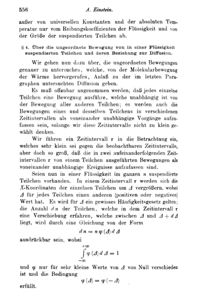
§4, paragraph 2: Each particle is assumed to move independently of all the others, and the motions of one particle in different time intervals count as independent too, as long as the intervals are not taken too small.
§4, paragraph 3: He introduces a time interval τ, very small compared with the intervals one can observe, but long enough that a particle's motions in two successive intervals are independent events.
§4, paragraph 10: The mean displacement therefore grows as the square root of the time, and the root mean square of the total displacement in space is λx times the square root of 3.

Write the displacement after n steps as the sum of their increments. Expanding its square exposes both the squared increments and their cross terms. Independence factors each expected cross term into the product of two means; centring makes that product zero.

\left\langle \left(\sum_{i=1}^{n} \Delta_{i}\right)^{2}\right\rangle = \sum_{i=1}^{n} \left\langle \Delta_{i}^{2}\right\rangle = n\,l^{2}

Shown in modern letters; Einstein's are in §4 of the German source face.

The mean square of the sum of independent centred increments is the sum of their mean squares.

t = n\,\tau

D = \frac{l^{2}}{2\,\tau}

\left\langle x^{2}\right\rangle = 2\,D\,t

Shown in modern letters; Einstein's are in §4 of the German source face.

Elapsed time is n tau; defining D as ell squared over two tau gives mean-square displacement two D t.

Open the foundation: Probability and independence

Show every step here: Why the square grows with time

A tool for this step

Probability and independence

When you square a sum of random steps, why do the mixed terms average to zero?

Flip a coin twice and take one step for each flip: a metre to the right for heads, a metre to the left for tails. How far from the start do you end up, on average?

The four outcomes, right-right, right-left, left-right and left-left, are equally likely: one chance in four each.
They leave you 2 m to the right, back at the start, back at the start, or 2 m to the left.
Square those distances so that left and right count alike: 4, 0, 0 and 4. Their average is 2, one square metre for each step.

Combining the two steps added nothing beyond one square metre each. In symbols, with Δ₁ and Δ₂ for the two steps, squaring the sum gives each step squared and a mixed term, twice their product:

\left(\Delta_{1} + \Delta_{2}\right)^{2} = \Delta_{1}^{2} + 2\,\Delta_{1}\,\Delta_{2} + \Delta_{2}^{2}

Delta one plus delta two, squared, equals delta one squared plus two delta one delta two plus delta two squared.

In the coin walk the product of the two steps is +1 for right-right and left-left and −1 for the other two, so on average it is zero and the mixed term adds nothing. Two conditions make that happen. Independence: learning the first step does not change the chances for the second, so the chance of a pair is the product of the two chances. Centring: each step averages zero, left as likely as right. Then the average of the product is the product of the averages, zero times zero:

\langle \Delta_1 \Delta_2 \rangle = \langle \Delta_1 \rangle \langle \Delta_2 \rangle = 0

The average of delta one times delta two equals the average of delta one times the average of delta two, which is zero.

Both conditions matter. If each step drifts, averaging +1, the product of the averages is 1, not 0. If the second step tends to copy the first, the product is positive more often than negative. The Brownian paper's §4 assumes that a particle's motions in successive intervals are independent, as long as the intervals are not chosen too small.

Worked example: What changes when the second step copies the first

Now let the second flip always copy the first. Only right-right and left-left can happen, one chance in two each.
The product of the two steps is +1 every time, so the mixed term no longer averages zero.
You always end 2 m from the start, so the squared distance is 4 every time: the average is 4, not 2. Independence removed that extra 2.

Where this lesson stops

Before dropping a mixed term, ask two things: does learning one step change the chances for the next, and does each step average zero?

Name the pieces. A tracer takes $n$ steps, one in each interval of time $\tau$ . Its $i$ -th step is a signed displacement $\Delta_i$ , where $i$ counts the steps 1, 2, 3 and so on up to $n$ . Where it ends, measured from where it started, is the sum of its steps: $x = \Delta_1 + \Delta_2 + \ldots + \Delta_n$ .
The assumptions, stated once. Each step is centred: its average over many tracers is zero, $\langle\Delta_i\rangle = 0$ , so on average it goes neither left nor right. Every step has the same mean square, written $l^2$ , so $l$ is the root-mean-square length of one step. And the steps are independent: knowing one step tells you nothing about any other.
Start with two steps and call them $A$ and $B$ . The square of their sum is found by multiplying it out, $(A+B)(A+B)$ , which gives four products, two of which are the same:

\left(A + B\right)^{2} = A^{2} + 2\,A\,B + B^{2}

Shown in modern letters; Einstein's are in §4 of the German source face.

The square of A plus B contains two squares and twice the cross product.

Average both sides over many tracers. The average of a sum is the sum of the averages, and a fixed number such as 2 can be taken outside an average, so $\langle(A+B)^2\rangle = \langle A^2\rangle + 2\langle AB\rangle + \langle B^2\rangle$ .
The middle term is where independence enters. For independent steps, the average of a product is the product of the averages: $\langle AB\rangle = \langle A\rangle\langle B\rangle$ . Both steps are centred, so both averages are zero, and $\langle AB\rangle = 0$ .
Check this with the simplest walk, where each step is +1 or −1 with equal chance. The four equally likely pairs (+1, +1), (+1, −1), (−1, +1) and (−1, −1) give the products +1, −1, −1, +1, whose average is zero. The squares $A^2$ and $B^2$ are always 1, so the mean square after two steps is 1 + 0 + 1 = 2.
Three steps work the same way. Multiplying out $(\Delta_1+\Delta_2+\Delta_3)^2$ gives three squares, $\Delta_1^2 + \Delta_2^2 + \Delta_3^2$ , and three cross terms, $2\Delta_1\Delta_2 + 2\Delta_1\Delta_3 + 2\Delta_2\Delta_3$ , one for each pair of different steps. Each cross term averages to zero, for the reason just given.
For $n$ steps there are $n$ squares and one cross term for every pair of different steps. Every cross term averages to zero. Each square averages to $l^2$ , so the $n$ squares together contribute $n$ times $l^2$ . In symbols, where $\sum_{i=1}^n$ means add up for $i$ from 1 to $n$ :

\left\langle \left(\sum_{i=1}^{n} \Delta_{i}\right)^{2}\right\rangle = \sum_{i=1}^{n} \left\langle \Delta_{i}^{2}\right\rangle = n\,l^{2}

Shown in modern letters; Einstein's are in §4 of the German source face.

The mean square of the sum of independent centred increments is the sum of their mean squares.

Now bring in time. Each step takes the interval $\tau$ , so after $n$ steps the elapsed time is $t = n\tau$ . Dividing both sides by $\tau$ , the number of steps is $n = t/\tau$ .
Replace $n$ in the mean square: $\langle x^2\rangle = nl^2 = (t/\tau)\,l^2$ . Regroup the same factors as $(l^2/\tau)\,t$ : a constant times the elapsed time.
Write the constant $l^2/\tau$ as 2 times $l^2/(2\tau)$ , and give $l^2/(2\tau)$ its own name, $D$ , the diffusivity of the walk. The factor 2 is a choice of convention: with it, this $D$ is the same coefficient that appears in the diffusion equation of the next passage. The three statements together:

t = n\,\tau

D = \frac{l^{2}}{2\,\tau}

\left\langle x^{2}\right\rangle = 2\,D\,t

Shown in modern letters; Einstein's are in §4 of the German source face.

Elapsed time is n tau; defining D as ell squared over two tau gives mean-square displacement two D t.

The mean square grows in proportion to time: four times the time gives four times the mean square. The RMS is its square root, and $\sqrt{4} = 2$ , so four times the time gives twice the RMS, not four times. In the ±1 walk, 4 steps give a mean square of 4 and an RMS of 2; 16 steps give a mean square of 16 and an RMS of 4.
Each assumption did work. If the steps were not centred, $\langle A\rangle\langle B\rangle$ would not vanish, and the cross terms would add a part growing like $n^2$ , the square of a steady drift. If the steps were not independent, $\langle AB\rangle$ need not factor at all. If the mean square of a step were infinite, there would be no $l^2$ to add.

A tool for this step

From steps to spread

Why does typical displacement grow as the square root of the step count?

A walker flips a coin before every step: heads, one metre to the right; tails, one metre to the left. After four steps, how far from the start is the walker likely to be? Not four metres: the steps partly cancel. Count the walks, and square each final distance so that left and right count alike:

After one step the walker is 1 m away, every time. The squared distance is 1.
After two steps there are four equally likely walks, ending 2 m right, at the start, at the start, or 2 m left. The squared distances 4, 0, 0 and 4 average 2.
After four steps there are sixteen equally likely walks. Two end 4 m out, eight end 2 m out and six end at the start. The squared distances average (2 × 16 + 8 × 4) ÷ 16 = 4.

The average squared distance grows by one square metre per step: after n steps it is n. The typical distance, its square root, grows only as the square root of n: 1 m after one step, about 1.4 m after two, 2 m after four, 10 m after a hundred. To get twice as far takes four times as many steps.

In symbols, call the steps Δ₁, Δ₂ and so on, and the position after n steps X, their sum:

X_n=\Delta_1+\ldots+\Delta_n

Position after n steps is the sum of the n signed increments.

Suppose each step averages zero and has the same mean square l², where l is the typical size of one step (1 m in the coin walk). Squaring the sum gives the n squared steps and many products of two different steps. When the steps are independent and each averages zero, every such product averages zero, as the lesson on independence shows for two coin steps. Only the squares are left to add up:

\left\langle X_{n}^{2}\right\rangle = n\,l^{2}

\sqrt{\left\langle X_{n}^{2}\right\rangle} = l\,\sqrt{n}

The mean square is n times ell squared, and RMS displacement is ell times the square root of n.

Worked example: A hundred steps, then four hundred

A hundred steps of typical size 1 m leave a typical distance of 10 m from the start, because the square root of 100 is 10. Four hundred steps leave 20 m: four times the steps, twice the distance. No single walker has to end exactly 10 or 20 m away; these are typical sizes over many walkers. Nor is the distance from the start the length of the path: to end 10 m from home, the walker has walked 100 m.

Four steps is not four metres

The four two-step walks the lesson lists, each drawn from the start. Two arrows a walk, and a dot where it ends.

The four ends add to zero, so the average end is the start. Their squares are 4, 0, 0, 4, which add to 8 and average 2. Squares do not cancel, and that is the quantity that keeps count.

So the typical distance climbs, but slowly. The straight line is what a reader expects before reading the lesson: every step in the same direction.

What it shows, in words

The first drawing is the four equally likely two-step walks. Right then right ends 2 metres right; right then left and left then right both end back at the start; left then left ends 2 metres left. The four ends add to zero, so the average end is the start, and nobody should read that as the walker not having moved. The squares of those ends are 4, 0, 0, 4, and their average is 2 square metres, which is two step-squares for two steps.

The second drawing is the typical distance against the number of steps. It passes through 1 metre at 1 step, 2 at 4, 3 at 9 and 4 at 16: four times the steps for twice the distance, every time. The broken straight line is a walker whose every step went the same way, one metre per step, and it leaves the top of the graph after 5 steps. At a hundred steps the curve is at 10 metres where that line would be at a hundred.

Where this lesson stops

The coin walk is a picture, not a claim that molecules push a particle in fixed jumps. The Brownian paper needs only that the particle's moves in successive intervals are independent of one another.

Why the mean square is tractable

Choose a transition to open its explanation. Without JavaScript, open the worked bridge below; it contains the same four explanations.

Expand the square
Average each contribution
Why do the cross terms vanish?
Add equal mean squares

Read all four transitions here (also works without JavaScript)

Expand the square

Pedagogical bridge, not the paper’s printed calculation

Expand the square

This is newly authored explanatory prose, not the German text or a translation. The two-step calculation below illustrates the pairwise argument for any finite number of steps.

Changed subexpression: the total mean-square expression. The outline marks it on both sides.

Before

\htmlData{expression-id=totalMeanSquare}{\boxed{\left\langle \left(A + B\right)^{2}\right\rangle}}

After

\htmlData{expression-id=totalMeanSquare}{\boxed{\left\langle A^{2} + 2\,A\,B + B^{2}\right\rangle}}

Rule: Expand algebraic terms: use the stated equality without changing its assumptions.

Open the mathematical tool behind this step →

Expand (A + B)² as A² + 2AB + B² before averaging. The 2AB term records how the two steps combine.

In fewer words

Two added steps produce three kinds of term, not just two squares.

Show every step in this transition

This algebra holds for every pair of step values, even correlated or biased ones. No probability assumption has been used yet.

What this step assumes

No new independence or centring premise is used at this step. The averages are assumed to exist.

Treat increments over the chosen intervals as independent, centred, and having the same finite second moment. In a Brownian model this is a coarse-grained assumption, not a claim about arbitrarily short times.

Two signed steps: see every possible outcome

Each step is +1 or −1 in arbitrary step units. Rows have equal probability within each selected model. These are exact finite teaching distributions, not observations or simulated Brownian paths.

Independent steps

All four pairs are equally likely. The cross products cancel only in the average, not in each outcome.

4 equally likely outcomes. Squared columns use squared step units.
A	B	A + B	(A + B)²	A² + B²	2AB
-1	-1	-2	4	2	2
1	-1	0	0	2	-2
-1	1	0	0	2	-2
1	1	2	4	2	2

Mean square: 2. Mean cross contribution: 0. Signed mean: 0. Mean absolute displacement: 1.

Always the same direction

Both individual steps still have zero mean and mean square one. Removing independence makes the cross contribution positive.

2 equally likely outcomes. Squared columns use squared step units.
A	B	A + B	(A + B)²	A² + B²	2AB
-1	-1	-2	4	2	2
1	1	2	4	2	2

Mean square: 4. Mean cross contribution: 2. Signed mean: 0. Mean absolute displacement: 2.

Always opposite directions

The same individual step averages now produce complete cancellation of the total displacement. Zero means alone are not enough.

2 equally likely outcomes. Squared columns use squared step units.
A	B	A + B	(A + B)²	A² + B²	2AB
-1	1	0	0	2	-2
1	-1	0	0	2	-2

Mean square: 0. Mean cross contribution: -2. Signed mean: 0. Mean absolute displacement: 0.

From two steps to many

For n steps, expand the square of their sum. There are n individual squared terms and cross terms for distinct pairs. Every cross average vanishes under independence and zero mean; equal step mean squares then give n times the one-step mean square. With t = nτ and D defined as the one-step mean square divided by 2τ, the result is 2Dt.

The mean absolute displacement is not a wrong answer. It also measures spreading, but absolute value does not distribute over addition, so it lacks this simple additive calculation. Neither absolute displacement nor RMS displacement is total path length.

Modern lens: where the independence model stops

Modern lens: inertia introduces a short-time regime in which successive motions need not be independent. Momentum relaxation time is a later dynamical interpretation, not a premise used in this teaching derivation.

Compare the paper’s step-distribution route (explanation preview) →

Average each contribution

Pedagogical bridge, not the paper’s printed calculation

Average each contribution

This is newly authored explanatory prose, not the German text or a translation. The two-step calculation below illustrates the pairwise argument for any finite number of steps.

Changed subexpression: the total mean-square expression. The outline marks it on both sides.

Before

\htmlData{expression-id=totalMeanSquare}{\boxed{\left\langle A^{2} + 2\,A\,B + B^{2}\right\rangle}}

After

\htmlData{expression-id=totalMeanSquare}{\boxed{\begin{aligned}& \left\langle A^{2}\right\rangle \\ &{}+ \left(\left\langle 2\,A\,B\right\rangle\right) \\ &{}+ \left\langle B^{2}\right\rangle\end{aligned}}}

Rule: Linearity of averaging: average the sum by adding the averages. Independence is not required for this move.

Open the mathematical tool behind this step →

Apply linearity of expectation to the two squared terms and the cross term. Linearity does not require independence.

In fewer words

Averaging a sum is the same as adding its averages.

Show every step in this transition

Finite second moments ensure these averages exist. Expectation distributes over addition and a fixed multiplier: ⟨A² + 2AB + B²⟩ = ⟨A²⟩ + 2⟨AB⟩ + ⟨B²⟩.

What this step assumes

No new independence or centring premise is used at this step. The averages are assumed to exist.

Two signed steps: see every possible outcome

Each step is +1 or −1 in arbitrary step units. Rows have equal probability within each selected model. These are exact finite teaching distributions, not observations or simulated Brownian paths.

Independent steps

All four pairs are equally likely. The cross products cancel only in the average, not in each outcome.

4 equally likely outcomes. Squared columns use squared step units.
A	B	A + B	(A + B)²	A² + B²	2AB
-1	-1	-2	4	2	2
1	-1	0	0	2	-2
-1	1	0	0	2	-2
1	1	2	4	2	2

Mean square: 2. Mean cross contribution: 0. Signed mean: 0. Mean absolute displacement: 1.

Always the same direction

Both individual steps still have zero mean and mean square one. Removing independence makes the cross contribution positive.

2 equally likely outcomes. Squared columns use squared step units.
A	B	A + B	(A + B)²	A² + B²	2AB
-1	-1	-2	4	2	2
1	1	2	4	2	2

Mean square: 4. Mean cross contribution: 2. Signed mean: 0. Mean absolute displacement: 2.

Always opposite directions

The same individual step averages now produce complete cancellation of the total displacement. Zero means alone are not enough.

2 equally likely outcomes. Squared columns use squared step units.
A	B	A + B	(A + B)²	A² + B²	2AB
-1	1	0	0	2	-2
1	-1	0	0	2	-2

Mean square: 0. Mean cross contribution: -2. Signed mean: 0. Mean absolute displacement: 0.

From two steps to many

Modern lens: where the independence model stops

Compare the paper’s step-distribution route (explanation preview) →

Why do the cross terms vanish?

Pedagogical bridge, not the paper’s printed calculation

Why do the cross terms vanish?

This is newly authored explanatory prose, not the German text or a translation. The two-step calculation below illustrates the pairwise argument for any finite number of steps.

The move: cross terms average away, not individual displacements.

Changed subexpression: the cross-term average. The outline marks it on both sides.

Before

\begin{aligned}& \left\langle A^{2}\right\rangle \\ &{}+ \htmlData{expression-id=crossTerm}{\boxed{\left(\left\langle 2\,A\,B\right\rangle\right)}} \\ &{}+ \left\langle B^{2}\right\rangle\end{aligned}

After

\left\langle A^{2}\right\rangle + \htmlData{expression-id=crossTerm}{\boxed{\left(0\right)}} + \left\langle B^{2}\right\rangle

Rule: For independent, zero-mean quantities, the mean of their product is the product of their means, hence zero.

Open the mathematical tool behind this step →

Independence gives ⟨AB⟩ = ⟨A⟩⟨B⟩. The two means are zero, so the average cross term is zero. It is not zero in each individual outcome.

In fewer words

Independent, unbiased steps have no average cross contribution.

Show every step in this transition

These are two separate premises. Zero marginal means alone do not force ⟨AB⟩ to vanish: when B always equals A, both means are zero but AB is always positive. Pairwise uncorrelated zero-mean steps would also suffice; independence is the stronger premise used here.

What this step assumes

The increments A and B are independent.
Each increment has mean zero.

Two signed steps: see every possible outcome

Each step is +1 or −1 in arbitrary step units. Rows have equal probability within each selected model. These are exact finite teaching distributions, not observations or simulated Brownian paths.

Independent steps

All four pairs are equally likely. The cross products cancel only in the average, not in each outcome.

4 equally likely outcomes. Squared columns use squared step units.
A	B	A + B	(A + B)²	A² + B²	2AB
-1	-1	-2	4	2	2
1	-1	0	0	2	-2
-1	1	0	0	2	-2
1	1	2	4	2	2

Mean square: 2. Mean cross contribution: 0. Signed mean: 0. Mean absolute displacement: 1.

Always the same direction

Both individual steps still have zero mean and mean square one. Removing independence makes the cross contribution positive.

2 equally likely outcomes. Squared columns use squared step units.
A	B	A + B	(A + B)²	A² + B²	2AB
-1	-1	-2	4	2	2
1	1	2	4	2	2

Mean square: 4. Mean cross contribution: 2. Signed mean: 0. Mean absolute displacement: 2.

Always opposite directions

The same individual step averages now produce complete cancellation of the total displacement. Zero means alone are not enough.

2 equally likely outcomes. Squared columns use squared step units.
A	B	A + B	(A + B)²	A² + B²	2AB
-1	1	0	0	2	-2
1	-1	0	0	2	-2

Mean square: 0. Mean cross contribution: -2. Signed mean: 0. Mean absolute displacement: 0.

From two steps to many

Modern lens: where the independence model stops

Compare the paper’s step-distribution route (explanation preview) →

Add equal mean squares

Pedagogical bridge, not the paper’s printed calculation

Add equal mean squares

This is newly authored explanatory prose, not the German text or a translation. The two-step calculation below illustrates the pairwise argument for any finite number of steps.

Changed subexpression: the total mean-square expression. The outline marks it on both sides.

Before

\htmlData{expression-id=totalMeanSquare}{\boxed{\left\langle A^{2}\right\rangle + \left(0\right) + \left\langle B^{2}\right\rangle}}

After

\htmlData{expression-id=totalMeanSquare}{\boxed{2\,l^{2}}}

Rule: Substitution: use the stated equality without changing its assumptions.

Open the mathematical tool behind this step →

Here l² denotes the mean square of one step. The two remaining contributions are l² + l² = 2l².

In fewer words

Two equal contributions give twice one contribution.

Show every step in this transition

For n increments the expansion contains n square terms and one ordered cross term for every i ≠ j. The same independence and centring argument eliminates each cross average. If every step has mean square l², the result is nl².

What this step assumes

Each increment has the same finite mean square, called l² in this worked bridge.

Two signed steps: see every possible outcome

Each step is +1 or −1 in arbitrary step units. Rows have equal probability within each selected model. These are exact finite teaching distributions, not observations or simulated Brownian paths.

Independent steps

All four pairs are equally likely. The cross products cancel only in the average, not in each outcome.

4 equally likely outcomes. Squared columns use squared step units.
A	B	A + B	(A + B)²	A² + B²	2AB
-1	-1	-2	4	2	2
1	-1	0	0	2	-2
-1	1	0	0	2	-2
1	1	2	4	2	2

Mean square: 2. Mean cross contribution: 0. Signed mean: 0. Mean absolute displacement: 1.

Always the same direction

Both individual steps still have zero mean and mean square one. Removing independence makes the cross contribution positive.

2 equally likely outcomes. Squared columns use squared step units.
A	B	A + B	(A + B)²	A² + B²	2AB
-1	-1	-2	4	2	2
1	1	2	4	2	2

Mean square: 4. Mean cross contribution: 2. Signed mean: 0. Mean absolute displacement: 2.

Always opposite directions

The same individual step averages now produce complete cancellation of the total displacement. Zero means alone are not enough.

2 equally likely outcomes. Squared columns use squared step units.
A	B	A + B	(A + B)²	A² + B²	2AB
-1	1	0	0	2	-2
1	-1	0	0	2	-2

Mean square: 0. Mean cross contribution: -2. Signed mean: 0. Mean absolute displacement: 0.

From two steps to many

Modern lens: where the independence model stops

Compare the paper’s step-distribution route (explanation preview) →

Explore the equations in this step

Read each operation, check its units and assumptions, or open the mathematical step behind it. These are modern teaching equations, not the equations as printed.

Explore the equation · Modern model notation

The mean square grows in proportion to time

\left\langle x^{2}\right\rangle = 2\,D\,t

Shown in modern letters; Einstein's are in §4 of the German source face.

squared is two times times .

Select a term or operation. In the formula, Down enters an operation, Up returns to its parent, and Left/Right move between siblings. Escape clears selection. Tab leaves the formula.

Explain this equation

Each term and operation, in words

No live values

This equation states a relation. No instrument on this page computes its terms.

Read the equation aloud in words

The mean square displacement equals two D t.

The squares of independent steps add, so the mean square grows in proportion to time, not to its square.

Model assumptions and every term’s meaning

Independent, zero-mean steps.
These are modern teaching equations in SI notation, not a transcription of the printed paper.

The mean square: Averaged over many particles. Read the prerequisite
Two D t: Linear in time. Read the prerequisite
What it asserts: Four times as long gives four times the mean square. Read the prerequisite
x squared: Squared, so both directions count. Read the prerequisite
Diffusion coefficient: How fast the mean square displacement grows: half its rate of growth. Not a speed. Read the prerequisite
Displacement since the start: How far one particle has moved along x since observation began. Read the prerequisite
Observation interval: The time over which displacement is observed. Read the prerequisite

Every term’s units were checked when this page was built. That checks the units, not the model. This equation is written for this edition in modern notation, not transcribed from the paper.

Explore the equation · Modern model notation

The square of a sum

\left(A + B\right)^{2} = A^{2} + 2\,A\,B + B^{2}

Shown in modern letters; Einstein's are in §4 of the German source face.

plus , squared, is squared plus two plus squared.

Select a term or operation. In the formula, Down enters an operation, Up returns to its parent, and Left/Right move between siblings. Escape clears selection. Tab leaves the formula.

Explain this equation

Each term and operation, in words

No live values

This equation states a relation. No instrument on this page computes its terms.

Read the equation aloud in words

A plus B, squared, equals A squared plus two A B plus B squared.

The cross term 2AB is what averages to zero when the next step is independent of the ones before it, which is why the mean squares simply add.

Model assumptions and every term’s meaning

Ordinary algebra; A and B are any numbers.
These are modern teaching equations in SI notation, not a transcription of the printed paper.

A squared: A times A. Read the prerequisite
B squared: B times B. Read the prerequisite
The cross term: Twice A times B: it vanishes on average for an independent, zero-mean B. Read the prerequisite
Three terms: Each term of the bracket times each term. Read the prerequisite
What it asserts: An identity: true for every A and B. Read the prerequisite
The sum, squared: The whole bracket times itself, not each term squared. Read the prerequisite
A plus B: The sum to be squared. Read the prerequisite
Any number: A stands for any number; here, the sum of the earlier steps. Read the prerequisite
Any other number: B stands for any number; here, the next step. Read the prerequisite

Every term’s units were checked when this page was built. That checks the units, not the model. This equation is written for this edition in modern notation, not transcribed from the paper.

Explore the equation · Modern model notation

The mean square of n independent steps

\left\langle \left(\sum_{i=1}^{n} \Delta_{i}\right)^{2}\right\rangle = \sum_{i=1}^{n} \left\langle \Delta_{i}^{2}\right\rangle = n\,l^{2}

Shown in modern letters; Einstein's are in §4 of the German source face.

The mean square of the net displacement is the sum of the steps' mean squares: times squared.

Select a term or operation. In the formula, Down enters an operation, Up returns to its parent, and Left/Right move between siblings. Escape clears selection. Tab leaves the formula.

Explain this equation

Each term and operation, in words

No live values

This equation states a relation. No instrument on this page computes its terms.

Read the equation aloud in words

The mean of the square of the sum, for i from 1 to n, of Delta sub i, equals the sum, for i from 1 to n, of the mean of Delta sub i squared, which equals n l squared.

Square the sum of n steps and average. Every cross term between two different steps averages to zero, because the steps are independent and centred. Only the n squared steps remain, each contributing l squared.

Model assumptions and every term’s meaning

The n steps are independent, each with mean zero and the same mean square l squared.
These are modern teaching equations in SI notation, not a transcription of the printed paper.

Equal step sizes: Each step has the same mean square l squared, so n of them give n l squared. Read the prerequisite
The cross terms drop out: Independent, centred steps: every cross term averages to zero, leaving only the squares. Read the prerequisite
Mean square of the net displacement: The average, over many walkers, of the square of where each ends up. Read the prerequisite
Squared: The net displacement squared, so left and right count alike. Read the prerequisite
The net displacement: The n steps added, each with its sign. Read the prerequisite
Add the mean squares: The sum, over the n steps, of each step's mean square. Read the prerequisite
One step's mean square: The average of one step's square over many walkers. Read the prerequisite
A step squared: Step i squared. Read the prerequisite
n times: n equal contributions. Read the prerequisite
l squared: The mean square of one step. Read the prerequisite
Step i: Delta sub i: the i-th signed step of the walk. Read the prerequisite
Step i: The same Delta sub i. Read the prerequisite
Number of steps: n: how many independent steps the walk takes. Read the prerequisite
Number of steps: The same n. Read the prerequisite
Step length: l: the root mean square length of one step. Read the prerequisite

Every term’s units were checked when this page was built. That checks the units, not the model. This equation is written for this edition in modern notation, not transcribed from the paper.

Explore the equation · Modern model notation

The diffusivity of a walk

D = \frac{l^{2}}{2\,\tau}

Shown in modern letters; Einstein's are in §4 of the German source face.

is squared over two .

Select a term or operation. In the formula, Down enters an operation, Up returns to its parent, and Left/Right move between siblings. Escape clears selection. Tab leaves the formula.

Explain this equation

Each term and operation, in words

No live values

This equation states a relation. No instrument on this page computes its terms.

Read the equation aloud in words

D equals l squared over two tau.

A walk of steps of length l every tau spreads like diffusion with this D.

Model assumptions and every term’s meaning

Independent steps of mean square length l squared.
These are modern teaching equations in SI notation, not a transcription of the printed paper.

Two tau: The two is one dimension's convention. Read the prerequisite
Step square per unit time: Squared length per second. Read the prerequisite
What it asserts: The microscopic walk sets the macroscopic D. Read the prerequisite
l squared: The mean square of one step. Read the prerequisite
Diffusion coefficient: How fast the mean square displacement grows: half its rate of growth. Not a speed. Read the prerequisite
Step interval: The short time between successive steps of the walk. Read the prerequisite
Step length: The root mean square length of one step. Read the prerequisite

Every term’s units were checked when this page was built. That checks the units, not the model. This equation is written for this edition in modern notation, not transcribed from the paper.

Explore the equation · Modern model notation

Time counts steps

t = n\,\tau

Shown in modern letters; Einstein's are in §4 of the German source face.

is times .

Select a term or operation. In the formula, Down enters an operation, Up returns to its parent, and Left/Right move between siblings. Escape clears selection. Tab leaves the formula.

Explain this equation

Each term and operation, in words

No live values

This equation states a relation. No instrument on this page computes its terms.

Read the equation aloud in words

t equals n tau.

n steps of duration tau take time t.

Model assumptions and every term’s meaning

Steps of equal duration tau.
These are modern teaching equations in SI notation, not a transcription of the printed paper.

n times tau: The total time of n steps. Read the prerequisite
What it asserts: Counting steps and measuring time are the same thing here. Read the prerequisite
Number of steps: How many independent steps fit in time t. Read the prerequisite
Step interval: The short time between successive steps of the walk. Read the prerequisite
Observation interval: The time over which displacement is observed. Read the prerequisite

Every term’s units were checked when this page was built. That checks the units, not the model. This equation is written for this edition in modern notation, not transcribed from the paper.

Modern qualifications

Einstein’s independence holds over his interval $\tau$ , not at every instant: over very short times a particle’s velocity carries over from one moment to the next, which is why $\tau$ must not be too small. Paul Langevin’s equation of 1908, which keeps the particle’s inertia, shows where that crossover lies. A simulation that agrees with $2Dt$ checks the arithmetic of the model, not the existence of molecules.

Assumptions and limits: Why the square grows with time

Assumed here

Increments are independent, have zero mean, and share a finite mean square ℓ².
One step corresponds to a declared interval τ.

What this does not establish

Correlated steps, bias or an infinite second moment change the argument.
This pedagogical walk does not describe fixed physical jumps in a liquid.

Earlier step: Zero average is not no movement

Source context: Annalen der Physik (4), 17, 549–560 (1905), §§1–5. Bibliographic pointer; this preview is not a source transcription or translation.

A derivation, to an approximation

From a step law to a density law

How can random individual steps produce a deterministic equation?

The 6 printed paragraphs this passage explains

§4, paragraph 1: Einstein now examines more closely the irregular motions, brought about by the thermal motion of the molecules, that give rise to the diffusion of §3.
§4, paragraph 3: He introduces a time interval τ, very small compared with the intervals one can observe, but long enough that a particle's motions in two successive intervals are independent events.
§4, paragraph 4: In each interval τ every particle's x coordinate changes by some amount Δ, positive or negative; the number of particles with a change between Δ and Δ + dΔ is n φ(Δ) dΔ, where φ adds up to one over all Δ, is non-zero only for very small Δ, and is the same for Δ and −Δ.
§4, paragraph 5: He asks how the diffusion coefficient depends on φ, again restricting himself to a number of particles per unit volume that depends only on x and t.
§4, paragraph 6: Calling that number f(x, t), he expresses the particles present at time t + τ through those present at time t, expands for small τ and small Δ, drops the terms that vanish by symmetry or are very small, and, calling the mean square jump divided by twice τ the quantity D, obtains equation (1): the rate of change of f in time equals D times its second derivative in x.
§4, paragraph 7: This is the known differential equation of diffusion, and D is recognised as the diffusion coefficient.

Let $\varphi(\Delta)$ be the probability density for a displacement $\Delta$ during $\tau$ . To end at $x$ , a tracer must start at $x - \Delta$ and then make that displacement. Adding over all possible increments gives the transition relation, written here in modern notation.

\begin{aligned}& p\left(x,\,t + \tau\right) \\ &\qquad \mathrel{=} \int_{-\infty}^{\infty} p\left(x - \Delta,\,t\right)\,\varphi\left(\Delta\right)\,\mathrm{d}\Delta\end{aligned}

Shown in modern letters; Einstein's are in §4 of the German source face.

The density one interval later is the integral, over every jump, of the density one jump away now, times how likely that jump is.

Expand to first order in time and second order in displacement. Normalization cancels the zeroth-order term. Symmetry removes the first moment. The second moment remains.

D = \frac{1}{2\,\tau}\,\int_{-\infty}^{\infty} \Delta^{2}\,\varphi\left(\Delta\right)\,\mathrm{d}\Delta

D is half the mean-square step divided by the step interval.

\frac{\partial p}{\partial t} = D\,\frac{\partial^{2} p}{\partial x^{2}}

Shown in modern letters; Einstein's are in §4 of the German source face.

The retained equation is the diffusion equation.

Open the foundation: Approximating a curve near a point

Show every step here: From a step law to a density law

A tool for this step

Approximating a curve near a point

Why can a curve be replaced, close to one point, by a few simple terms?

What is 2.1 squared, without a calculator? Start from what you know: 2 squared is 4. Picture a square 2 wide growing to 2.1 wide. It gains two strips, each 2 long and 0.1 thick, which add 0.4, and a small corner, 0.1 by 0.1, which adds 0.01. So 2.1 squared is 4.41. The first correction, 0.4, did almost all the work; the second, 0.01, is forty times smaller.

The same recipe works for any smooth curve, close to a point where you know it. Start with its value there. Add its slope times the step Δ: the slope, or first derivative, is the change in output per unit of input. Then add half its curvature times Δ²: the curvature, or second derivative, says how fast the slope itself changes. Further terms carry higher powers of Δ, so they are small only when Δ is:

\begin{aligned}f(x+\Delta)&=f(x)+\Delta f'(x)\\&\quad+\frac{\Delta^2}{2}f''(x)+\ldots\end{aligned}

The value a step delta away equals the value, plus delta times the slope, plus half of delta squared times the curvature, plus further terms.

The Brownian paper does exactly this in §4. It expands the number of particles at x + Δ in powers of the jump Δ and keeps the terms up to Δ², because only very small jumps contribute and each further surviving term is much smaller than the one before. The Δ term averages away, since jumps to the left and to the right are equally likely, and the Δ² term becomes the diffusion coefficient. A real particle does not make independent jumps over arbitrarily short times, so the expansion holds for times long enough for successive jumps to be independent and short enough for each jump to be small.

Worked example: What the dropped term costs

\left(x + \Delta\right)^{2} = x^{2} + 2\,x\,\Delta + \Delta^{2}

For the square function, the local expansion is exact through the quadratic term.

Keep only the value and the slope term, 4 + 2 × 2 × Δ, and see what dropping Δ² costs as the step grows:

Δ = 0.1: 4.4 instead of 4.41. The error, 0.01, is about 0.2 per cent.
Δ = 0.5: 6 instead of 6.25. The error, 0.25, is 4 per cent.
Δ = 2: 12 instead of 16. The error, 4, is a quarter of the answer.
Halving the step quarters the error, because the dropped term is Δ².

The square, its two strips and its corner

A square 2 wide grown to 2.1, drawn to scale. The strips are a twentieth of the side and the corner is what the straight-line estimate throws away.

Keeping the square and the strips gives 4.4, which is the straight-line estimate. The whole grown square is 4.41. The difference is the corner, 0.01, and it did about a fiftieth of the work the strips did.

Now the same square at each step the lesson lists, all three at one scale. The corner grows as the square of the step, so it catches up quickly.

What it shows, in words

The first drawing is a square of side 2 and area 4, grown to 2.1. It gains a strip along its right edge and another along its top, each 2 long and 0.1 thick, which together add 0.4, and a small square corner of 0.1 by 0.1, which adds 0.01. Together that is 4.41. Everything is at its true size, so the corner really is the speck it looks like: a four-hundredth of the area.

The second drawing is the same square grown by 0.1, 0.5, 2 in turn, all at one scale. The dropped corners are 0.01, 0.25, 4. At the smallest step the corner is a speck and the straight-line estimate is almost the whole answer; at a step of 2 the corner is a quarter of the square and the estimate has stopped being useful. Halving the step quarters the corner, because the corner is the step squared.

What it does not show: squaring is the case where the series stops of its own accord. A square has one corner and nothing after it, so keeping the value, the strips and the corner is not an approximation at all, it is the whole answer. For a curve that is not a square there are further terms behind the corner, each smaller than the last near the point and each growing faster away from it, and nothing here draws them.

Extension · The step the mass–energy paper takes

Try it: the Lorentz factor at low speed, term by term

The factor 1/√(1 − v²/c²) runs through relativity. It is now called γ; the relativity paper writes it β, with V for the speed of light. The mass–energy paper finds that a body's kinetic energy falls by L(1/√(1 − v²/V²) − 1) when it emits light of energy L, and then expands that bracket. Writing x = v²/c², Newton's binomial series gives:

(1 − x)−1/2 = 1 + ½ x + ⅜ x² + ⁵/₁₆ x³ + ³⁵/₁₂₈ x⁴ + …   (|x| < 1)

1. Moderate speeds: partial sums at v/c = 0.6 (x = 0.36)

At sixty percent the speed of light, x = 0.36. The exact value of γ − 1 is 1/√(1 − 0.36) − 1 = 1/0.8 − 1 = 0.25. Add the terms of the series one at a time and the total closes in on it:

Partial sums of γ − 1 at x = 0.36 against exact 0.25
Term added	Its value	Running total	Short of 0.25
½ x	0.180000	0.180000	0.070000
⅜ x²	0.048600	0.228600	0.021400
⁵/₁₆ x³	0.014580	0.243180	0.006820
³⁵/₁₂₈ x⁴	0.004593	0.247773	0.002227

Keeping only the first term is the paper's own step: "neglecting quantities of fourth and higher order", it writes the loss of kinetic energy as (L/V²)(v²/2). At v = 0.6c that gives 0.18L where the exact bracket gives 0.25L. The paper needs only low speeds, where the neglected terms are tiny.

2. Low speeds: a computer is also better off with the series

At v/c = 10⁻⁴, about 30 kilometres per second, roughly the Earth's speed round the Sun, x = 10⁻⁸ and γ = 1.000000005. A computer keeps about 16 significant digits, so subtracting 1 from γ throws away the first eight and leaves an answer made mostly of rounding error. The first term of the series, or the bracket rearranged so that nothing close to 1 is subtracted, keeps every digit:

Comparison at v/c = 10⁻⁴ (x = 10⁻⁸)

First series term (½ x):: 5.0000000000 × 10⁻⁹
Rearranged, nothing near 1 subtracted:: 5.0000000375 × 10⁻⁹
Its difference from the first term, relative:: 7.500000 × 10⁻⁹, which the next term predicts: 0.75x
Direct subtraction, 1/√(1 − x) − 1:: 5.0000001917 × 10⁻⁹
Its difference from the first term, relative:: 3.833145 × 10⁻⁸, about five times the true difference

The rearrangement: γ − 1 = x / (√(1 − x) · (1 + √(1 − x))). It is the same number as 1/√(1 − x) − 1, written so that no two nearly equal quantities are subtracted. At low speed, direct subtraction gets the eighth significant figure wrong; the rearrangement and the series do not.

Where this lesson stops

An expansion is a claim about size. Say which terms you keep, and why the ones you drop are smaller: here, because they carry higher powers of a small step.

Name the pieces. $p(x,t)$ is the density of tracers at position $x$ and time $t$ : the chance of finding a tracer between $x$ and a slightly larger $x + dx$ is $p(x,t)\,dx$ . Einstein writes this density as $f(x, t)$ and counts particles rather than chances; the steps below are the same for both.
$\tau$ is a short interval of time. During it each tracer moves by a signed displacement $\Delta$ , and $\varphi(\Delta)$ is the probability density of that displacement: the chance of a displacement between $\Delta$ and $\Delta + d\Delta$ is $\varphi(\Delta)\,d\Delta$ .
Two facts about $\varphi$ are assumed. It is normalized: some displacement certainly happens, so all its chances add up to one, $\int_{-\infty}^{\infty}\varphi(\Delta)\,d\Delta = 1$ . And it is symmetric: a jump to the left is as likely as the same jump to the right, $\varphi(-\Delta) = \varphi(\Delta)$ .
To be at $x$ at time $t + \tau$ , a tracer must have been at $x - \Delta$ at time $t$ and then made the displacement $\Delta$ . The chance of that one route is the density at its start times the chance of the jump, $p(x - \Delta, t)\,\varphi(\Delta)\,d\Delta$ , because in this model the jump law is the same wherever the tracer starts. Adding over every possible $\Delta$ , from far left to far right, gives the transition relation:

\begin{aligned}& p\left(x,\,t + \tau\right) \\ &\qquad \mathrel{=} \int_{-\infty}^{\infty} p\left(x - \Delta,\,t\right)\,\varphi\left(\Delta\right)\,\mathrm{d}\Delta\end{aligned}

Shown in modern letters; Einstein's are in §4 of the German source face.

The density one interval later is the integral, over every jump, of the density one jump away now, times how likely that jump is.

The integral sign $\int$ is that adding-up over every value of $\Delta$ . Both sides can now be simplified, using the assumption that $p$ changes little over one interval $\tau$ and over one jump $\Delta$ .
The left side, at fixed position. A short time $\tau$ later, the density is approximately its present value plus its rate of change in time, $\partial p/\partial t$ , multiplied by $\tau$ . The curly $\partial$ marks a partial derivative: a rate of change in one variable while the other is held fixed, here time with position held fixed.

p\left(x,\,t + \tau\right) \approx p\left(x,\,t\right) + \tau\,\frac{\partial p}{\partial t}

Shown in modern letters; Einstein's are in §4 of the German source face.

Keep the density and its first time change on the left.

The right side, at fixed time. The density a distance $\Delta$ to the left of $x$ is approximately its value at $x$ , minus the slope $\partial p/\partial x$ times $\Delta$ , plus half the curvature $\partial^2p/\partial x^2$ times $\Delta^2$ . The slope term carries a minus sign because the step is to the left. The curvature term does not, because $(-\Delta)^2 = \Delta^2$ . Here $p$ and its derivatives are all taken at $x$ and $t$ .

p\left(x - \Delta,\,t\right) \approx p - \Delta\,\frac{\partial p}{\partial x} + \frac{\Delta^{2}}{2}\,\frac{\partial^{2} p}{\partial x^{2}}

Shown in modern letters; Einstein's are in §4 of the German source face.

Keep value, slope and curvature of the spatial density on the right.

Put the spatial expansion into the integral and split it into three integrals, one for each term. The density and its derivatives are taken at $x$ , so they do not change as $\Delta$ runs over its values, and each one comes outside its integral.
First term: $p$ times $\int\varphi\,d\Delta$ , which is $p$ times one, because $\varphi$ is normalized.
Second term: $-\partial p/\partial x$ times $\int\Delta\varphi\,d\Delta$ . For a symmetric $\varphi$ , each positive $\Delta$ is matched by the negative $-\Delta$ with the same weight, so this integral is zero. That is why there is no drift.
Third term: $\frac{1}{2}\,\partial^2p/\partial x^2$ times $\int\Delta^2\varphi\,d\Delta$ . This integral is the mean-square jump. It is positive, because $\Delta^2$ is never negative, so symmetry cannot remove it.
Set the two sides equal: $p + \tau\,\partial p/\partial t \approx p + \frac{1}{2}\,\frac{\partial^2p}{\partial x^2}\int\Delta^2\varphi\,d\Delta$ . Subtract $p$ from both sides; normalization is what makes the two $p$ terms cancel. Then divide both sides by $\tau$ : $\partial p/\partial t$ is approximately $\frac{1}{2\tau}\int\Delta^2\varphi\,d\Delta$ times $\partial^2p/\partial x^2$ .
The factor in front of the curvature depends only on the jump law and on $\tau$ , not on $x$ or $t$ . Give it a name, $D$ :

D = \frac{1}{2\,\tau}\,\int_{-\infty}^{\infty} \Delta^{2}\,\varphi\left(\Delta\right)\,\mathrm{d}\Delta

D is half the mean-square step divided by the step interval.

It is the mean-square jump divided by $2\tau$ , the same form as the $l^2/(2\tau)$ of the previous passage. With that name, what remains is the diffusion equation:

\frac{\partial p}{\partial t} = D\,\frac{\partial^{2} p}{\partial x^{2}}

Shown in modern letters; Einstein's are in §4 of the German source face.

The retained equation is the diffusion equation.

Read it term by term. Where the density has a peak, its curvature is negative, so $\partial p/\partial t$ is negative and the peak falls. Where it has a hollow, the curvature is positive and the hollow fills. $D$ sets how fast.
What was dropped. The next spatial term carries $\Delta^3$ and vanishes by symmetry, like the $\Delta$ term. The first nonzero term left out carries $\Delta^4$ , and on the left the term with $\tau^2$ was left out. Cutting the expansion there is an approximation. It becomes exact only in a limit where the jumps shrink with the time step so that $D$ stays finite, and the equation describes the density on scales larger than one jump, not individual collisions.

A tool for this step

Adding continuously

How do you add up something that varies continuously?

Chance spread along a line is measured per unit length: a density. Where the density is the same all along a stretch, the chance of the stretch is the density times its length. A particle equally likely to be anywhere in a 4 µm stretch has density 0.25 per micrometre, and the chance of finding it in the first 1.5 µm is 0.25 × 1.5 = 0.375.

Where the density changes from place to place, cut the line into narrow strips. Each strip contributes its height times its width, as if the density were flat across it. Add the strips, then cut them narrower and add again. For a smooth curve the totals settle on one value, and that value is the integral:

\int_a^b p(x)\,dx = \lim_{\Delta x \to 0} \sum_i p(x_i)\,\Delta x

The integral of p of x from a to b is the value that the sum of p of x i times delta x settles on as delta x shrinks.

The units multiply. A probability density is a probability per metre, so a strip of it, times a width in metres, is a plain probability. For a density the whole area must be 1, because the particle has to be somewhere. The Brownian paper's §4 writes exactly that for the chances of a jump Δ, ∫φ(Δ) dΔ = 1, and the light-quanta paper's §3 adds entropy over every frequency, S = v∫φ dν.

One more tool recurs in the papers: integration by parts. It is the product rule for derivatives added up over an interval, and it moves a derivative from one factor to the other at the price of an endpoint term:

\int_a^b u\frac{dv}{dx}\,dx = [uv]_a^b - \int_a^b v\frac{du}{dx}\,dx

The integral of u times the derivative of v equals u v at b minus u v at a, minus the integral of v times the derivative of u.

The endpoint term, uv at b minus uv at a, is part of the answer. It disappears only when uv is zero at both ends, as it is for a density that falls to zero far out on both sides.

Worked example: A rising density, added up in narrower strips

A particle's density rises steadily across a 4 µm stretch, from 0 at the left end to 0.5 per micrometre at the right. The whole area is a triangle, ½ × 4 × 0.5 = 1.
Four strips 1 µm wide, each taking the height at its left edge: 0 + 0.125 + 0.25 + 0.375 = 0.75.
Eight strips 0.5 µm wide: the heights add to 1.75, and times 0.5 that is 0.875.
Sixteen strips 0.25 µm wide: 0.9375. The shortfall halves each time the strips do: 0.25, then 0.125, then 0.0625.
The totals settle on 1, the area of the triangle. That settled value is the integral.

A flat density gives the same total for every cut, which is why the uniform stretch above needed no strips. A curved one, such as the Brownian bell curve, does, and the integral is the value the totals settle on.

The same triangle, cut two ways

A density rising from 0 to 0.5 per micrometre across 4 μm. Each strip is as tall as the curve at its own left edge, which is why every strip falls short and why the shortfall shrinks when the strips do.

4 strips add to 0.75; 8 strips add to 0.875. The triangle itself is 1. Cut narrower and the total climbs toward it without ever passing it, and the value it climbs toward is the integral.

What it shows, in words

Both drawings are the same density, rising in a straight line from 0 at the left end to 0.5 per micrometre at the right, across 4 micrometres. The first is cut into 4 strips of 1 micrometre each and the second into 8 strips of 0.5.

Each strip is as tall as the line at its own left edge, so each leaves a wedge uncovered above it. The 4 strips add to 0.75 and the 8 strips to 0.875, against the triangle's area of 1. Narrower strips leave smaller wedges, so the totals climb toward 1 and never past it. That limit is what the integral names.

What it does not show: these strips take the height at their left edge, which is one choice among several. Taking the right edge would overshoot 1 and climb down to it instead, and taking the middle of each strip would land much closer from the start. All three settle on the same 1, and that they agree is the fact the integral rests on. Nothing in either drawing demonstrates it.

Where this lesson stops

An integral is a total of height times width over a range, in the units of both. The widths and any endpoint term are part of the calculation, not decoration on the integral sign.

A tool for this step

Partial derivatives and held-fixed quantities

When a quantity depends on two things, what does its rate of change mean?

The concentration of particles in a tube depends on where you look, x, and when you look, t. Ask how fast the concentration changes and there are two different answers: how it changes as you move along the tube at one instant, and how it changes at one place as time passes.

A partial derivative picks one of them. ∂f/∂x is the rate of change along the tube with the time t held fixed, like comparing points in one photograph. ∂f/∂t is the rate of change in time at a fixed position x, like watching one spot under the microscope. The curly ∂ says that something else is being held fixed, and a subscript names it:

\left(\frac{\partial f}{\partial x}\right)_t \qquad \left(\frac{\partial f}{\partial t}\right)_x

The partial derivative of f with respect to x at fixed t, and the partial derivative of f with respect to t at fixed x.

Thermodynamics depends on the same care. How much a gas's volume changes as the pressure changes depends on whether its temperature T is held fixed, with heat flowing in and out, or its entropy S is held fixed, with the gas insulated. The two derivatives have different values, and ∂V/∂p written alone does not say which is meant:

\left(\frac{\partial V}{\partial p}\right)_T \quad \text{versus} \quad \left(\frac{\partial V}{\partial p}\right)_S

The partial derivative of V with respect to p at fixed temperature T, versus the same derivative at fixed entropy S.

In §3 of the light-quanta paper, radiation fills a fixed volume and φ is its entropy per unit volume and per unit interval of frequency, a function of the energy density ρ and of ν. Varying ρ with the frequency ν held fixed, Einstein finds that the derivative is 1/T:

\left(\frac{\partial \varphi}{\partial \rho}\right)_{\nu} = \frac{1}{T}

The partial derivative of phi with respect to rho, at fixed frequency nu, equals one over T.

In §6 of the relativity paper, Maxwell's equations are rewritten in the coordinates ξ, η, ζ, τ of a moving system. A derivative with respect to x taken with y, z and t held fixed then becomes a combination of a derivative with respect to ξ and one with respect to τ, because holding the resting time t fixed does not hold the moving time τ fixed.

Worked example: The same diffusion profile, differentiated two ways

Take the spreading profile of the Brownian paper's §4, written for a single particle:

f\left(x,\,t\right) = \frac{1}{\sqrt{4\,\pi\,D\,t}}\,\exp\left(-\frac{x^{2}}{4\,D\,t}\right)

f of x and t equals one over the square root of four pi D t, times e to the minus x squared over four D t.

Hold t fixed and differentiate with respect to x. Only the exponent depends on x, and the derivative of −x²/4Dt with respect to x is −x/2Dt:

\left(\frac{\partial f}{\partial x}\right)_{t} = -\frac{x}{2\,D\,t}\,f\left(x,\,t\right)

The partial derivative of f with respect to x at fixed t equals minus x over two D t, times f.

That is the slope of the profile in one snapshot: downhill to the right of the centre, uphill to the left. Now hold x fixed and differentiate with respect to t. Both the factor in front and the exponent depend on t:

\left(\frac{\partial f}{\partial t}\right)_{x} = \left(-\frac{1}{2\,t} + \frac{x^{2}}{4\,D\,t^{2}}\right)\,f\left(x,\,t\right)

The partial derivative of f with respect to t at fixed x equals minus one over two t, plus x squared over four D t squared, all times f.

That is what a probe fixed at one place records. Near the centre, where x² is less than 2Dt, the bracket is negative: the concentration falls as the cloud spreads away. Farther out it is positive: the concentration rises as the cloud arrives. Differentiate the first result once more with respect to x and multiply by D, and you get the second. That is the §4 equation ∂f/∂t = D ∂²f/∂x², a rate at one place equal to a curvature at one time.

JavaScript is off, so the controls below cannot change anything. The construction shows its first setting, and its closing paragraph, “What it shows, in words”, describes the rest.

Try it: hold time fixed, or hold position fixed

In §4 of the Brownian paper, f(x, t) is the number of particles per unit volume at a place x along a tube, at a time t. “How fast does the concentration change?” then has two answers, and which one you mean depends on what you keep still: the moment, or the place.

Keep one of them still:

One moment: t fixed, ∂f/∂x

Freeze the moment and compare neighbouring places, as in a single photograph of the tube. ∂f/∂x says how steeply the concentration changes along it: particles per µm³ for each µm, which is particles per µm⁴.

Particles drift down that slope. The flux, the number crossing each square micrometre in a second, is J = −D ∂f/∂x: Fick’s first law.

One place: x fixed, ∂f/∂t

Keep your eye on one spot under the microscope and let time run. ∂f/∂t says how fast the count there rises or falls: particles per µm³ for each second.

Particles are neither made nor destroyed, so the count at a spot changes only by what flows in and out: ∂f/∂t = −∂J/∂x = D ∂²f/∂x². That is the diffusion equation of §4.

The same question in thermodynamics

Squeeze a gas and its pressure rises, but by how much depends on what else you keep fixed:

Three derivatives of pressure, and what each holds fixed
Held fixed	Derivative	What happens
Temperature T (isothermal)	(∂p / ∂V)_T	Heat flows in or out to keep the temperature constant.
Entropy S: no heat exchanged (adiabatic)	(∂p / ∂V)_S	The gas warms as it is squeezed, so its pressure climbs faster than at fixed temperature.
Volume V (isochoric)	(∂p / ∂T)_V	In a rigid vessel the pressure rises as the gas is heated.

What it shows, in words

∂f/∂x compares places at one moment; ∂f/∂t follows one place through time. They answer different questions and carry different units. In thermodynamics a subscript names what is held fixed, so (∂p/∂V)_T and (∂p/∂V)_S are different numbers for the same gas.

Where this lesson stops

A partial derivative is not defined until you have said which quantities are held fixed.

A tool for this step

What the diffusion coefficient means

What changes when D changes?

Put a drop of dye into a long tube of still water. At first the dye sits in one spot; an hour later it has spread along the tube, thinner and wider. The diffusion coefficient D says how fast that spreading goes.

The rule it follows is local. Look at one spot. If the dye is thicker on both sides than at the spot itself, a dip, dye drifts in from both sides and the spot fills. If the spot is a peak, thicker than its neighbours, dye drifts out and it thins. The more sharply the dip or peak is curved, the faster it changes, and D sets the pace. With p for how much dye sits per metre of tube at place x and time t:

\frac{\partial p}{\partial t} = D\,\frac{\partial^{2} p}{\partial x^{2}}

The time rate of change of density is D times its spatial curvature.

The right-hand side is D times the curvature, which is positive at a dip and negative at a peak. For one particle instead of a drop of dye, p is the probability per metre of finding it at x. Where the tube ends matters too: a closed tube keeps all its dye, and after a long time spreads it evenly, not in the ever-widening bell of an endless tube.

The same rule can be read as a flow. The amount crossing a point each second runs from thick to thin, faster where the density falls more steeply:

J = -D\,\frac{\partial p}{\partial x}

Fick’s constitutive law sends flux down the density gradient.

Combining the flux law with conservation gives the diffusion equation for constant D. The flux law itself is a model premise in this route, not something conservation alone proves.

Worked example: Doubling the diffusion coefficient, then quadrupling the time

Suppose the dye's typical distance from where it started is 1 mm after one minute. Double D, keeping everything else the same: the mean square doubles, so the typical distance becomes about 1.4 mm, the square root of 2 times as far, not twice. Keep the original D and wait four minutes instead of one: the typical distance doubles, to 2 mm. Neither comparison says where any single particle goes.

A peak empties, a dip fills

One profile of dye along the tube, thicker where the curve is higher. The arrows are what the rule does next at the two spots the lesson names.

The curvature is negative at the peak and positive at the dip. That is the whole of the sign in the rule: dye runs from thick to thin, and the two spots are one rule seen from two sides.

Later the same dye is wider and lower. The lesson's example: a typical distance of 1 mm after 1 minute.

What it shows, in words

The first drawing is one profile of dye with a peak a quarter of the way along the tube and a dip three quarters of the way along. At the peak the dye is thicker than on either side, so it leaves in both directions and the spot empties; at the dip it is thinner than on either side, so it arrives from both directions and the spot fills. Nothing in the picture treats the two spots differently: the same rule, that dye runs from thick to thin, empties one and fills the other.

The second drawing is the same dye at two times. After 1 minute its typical distance from the start is 1 mm; after four times as long it is 2 mm, twice as far, because the mean square grows with the time and the distance is its square root. Doubling the diffusion coefficient instead of the time would give about 1.4 mm, the square root of two rather than of four.

Where this lesson stops

D is measured in square metres per second. Before using it, say where the tube ends and what the model assumes, since both change the answer.

Explore the equations in this step

Read each operation, check its units and assumptions, or open the mathematical step behind it. These are modern teaching equations, not the equations as printed.

Explore the equation · Modern model notation

The diffusion equation

\frac{\partial p}{\partial t} = D\,\frac{\partial^{2} p}{\partial x^{2}}

Shown in modern letters; Einstein's are in §4 of the German source face.

in is times its second derivative along .

Select a term or operation. In the formula, Down enters an operation, Up returns to its parent, and Left/Right move between siblings. Escape clears selection. Tab leaves the formula.

Explain this equation

Each term and operation, in words

No live values

This equation states a relation. No instrument on this page computes its terms.

Read the equation aloud in words

The rate of change of the probability density with time equals D times its second derivative with respect to position.

Where the density curves upward it grows, and where it curves downward it falls, at a rate set by D. A peak therefore flattens and spreads.

Model assumptions and every term’s meaning

Independent steps with a symmetric step law and a finite mean square step.
Times long compared with one step, distances large compared with one step.
These are modern teaching equations in SI notation, not a transcription of the printed paper.

Curvature in space: The second derivative: how the slope of the density changes along x. Read the prerequisite
D times the curvature: The spreading rate: larger D, faster flattening. Read the prerequisite
Rate of change in time: How fast the density at one x changes. Read the prerequisite
What it asserts: The density changes in time exactly as fast as D times its curvature in space. Read the prerequisite
Probability density: Probability per metre of finding the particle at x after time t. Read the prerequisite
Diffusion coefficient: How fast the mean square displacement grows: half its rate of growth. Not a speed. Read the prerequisite
Position: The coordinate x along which the particles spread. Read the prerequisite
Time: The rate is per unit of time, at one fixed place x. Read the prerequisite

Every term’s units were checked when this page was built. That checks the units, not the model. This equation is written for this edition in modern notation, not transcribed from the paper.

Explore the equation · Modern model notation

The diffusion coefficient from the jumps

D = \frac{1}{2\,\tau}\,\int_{-\infty}^{\infty} \Delta^{2}\,\varphi\left(\Delta\right)\,\mathrm{d}\Delta

is one over two times the mean of the squared jump , each jump weighted by its density .

Select a term or operation. In the formula, Down enters an operation, Up returns to its parent, and Left/Right move between siblings. Escape clears selection. Tab leaves the formula.

Explain this equation

Each term and operation, in words

No live values

This equation states a relation. No instrument on this page computes its terms.

Read the equation aloud in words

D equals one over two tau times the integral, from minus infinity to infinity, of Delta squared times phi of Delta, d Delta.

D is the mean squared jump in one short interval, divided by twice that interval. Nothing about the fluid appears here yet; that comes with Stokes' law.

Model assumptions and every term’s meaning

Jumps in successive intervals are independent and symmetric, one coordinate.
These are modern teaching equations in SI notation, not a transcription of the printed paper.

Over every jump: Adds up the contribution of every possible jump, from any leftward to any rightward one. Read the prerequisite
Per two intervals: One over two tau turns a squared distance per jump into a rate. Read the prerequisite
Times: The rate factor times the averaged squared jump. Read the prerequisite
What it asserts: D is set by the jumps themselves: their mean square, per unit of time. Read the prerequisite
Jump squared: Squared, so leftward and rightward jumps both add. Read the prerequisite
Two tau: Twice the interval; the two comes from the second derivative of the density. Read the prerequisite
Weighted by how likely: Each squared jump counts in proportion to how often it happens. Read the prerequisite
How likely a jump is: Paper 2's phi: probability per metre of a jump of this size. A density, not a probability. Read the prerequisite
Diffusion coefficient: How fast the spread grows, in square metres per second. Not a speed. Read the prerequisite
The short interval: Paper 2's tau: short enough for the density to change little, long enough for jumps to be independent. Read the prerequisite
A jump: How far a particle moves in one interval tau. Read the prerequisite
The jump it describes: phi is read at this jump. Read the prerequisite
Summed over jumps: The variable the integral runs over. Read the prerequisite

Every term’s units were checked when this page was built. That checks the units, not the model. This equation is written for this edition in modern notation, not transcribed from the paper.

Explore the equation · Modern model notation

The density one interval later

\begin{aligned}& p\left(x,\,t + \tau\right) \\ &\qquad \mathrel{=} \int_{-\infty}^{\infty} p\left(x - \Delta,\,t\right)\,\varphi\left(\Delta\right)\,\mathrm{d}\Delta\end{aligned}

Shown in modern letters; Einstein's are in §4 of the German source face.

one later is the one away, weighted by , summed over every jump.

Select a term or operation. In the formula, Down enters an operation, Up returns to its parent, and Left/Right move between siblings. Escape clears selection. Tab leaves the formula.

Explain this equation

Each term and operation, in words

No live values

This equation states a relation. No instrument on this page computes its terms.

Read the equation aloud in words

p of x and t plus tau equals the integral, over every jump Delta from minus infinity to infinity, of p of x minus Delta and t, times phi of Delta.

A particle found at x after one more interval tau was somewhere else a jump earlier. Add up every jump Delta that could have brought it: the density at x minus Delta now, times how likely a jump of that size is.

Model assumptions and every term’s meaning

Jumps in successive intervals are independent, and the jump density phi is the same at every place and every time.
These are modern teaching equations in SI notation, not a transcription of the printed paper.

What it asserts: The density one interval later is fixed by the density now and the jump density alone. Read the prerequisite
One interval later: The time t plus one step interval tau: a later time, not a longer interval. Read the prerequisite
Over every jump: Adds up the arrivals from every possible jump, leftward and rightward. Read the prerequisite
Where it came from, times how likely: The density a jump away, weighted by the chance of that jump. Read the prerequisite
Where it came from: x minus Delta: the place a jump of Delta starts from if it ends at x. Read the prerequisite
The density later: Probability per metre of finding the particle at x, one interval after t. Read the prerequisite
Position: The place where the density is read. Read the prerequisite
Time: The time now. Every particle was at x = 0 when it read zero. Read the prerequisite
The step interval: Paper 2's tau: short, yet long enough for successive jumps to be independent. Read the prerequisite
The density now: The density at the starting place x minus Delta, at time t. Read the prerequisite
Position: The same x. Read the prerequisite
A jump: How far a particle moves in one interval tau. Read the prerequisite
Time: The same t: the density now. Read the prerequisite
How likely a jump is: Paper 2's phi: probability per metre of a jump of this size. Read the prerequisite
The jump it describes: phi is read at this jump. Read the prerequisite
Summed over jumps: The variable the integral runs over. Read the prerequisite

Every term’s units were checked when this page was built. That checks the units, not the model. This equation is written for this edition in modern notation, not transcribed from the paper.

Explore the equation · Modern model notation

The density one jump away

p\left(x - \Delta,\,t\right) \approx p - \Delta\,\frac{\partial p}{\partial x} + \frac{\Delta^{2}}{2}\,\frac{\partial^{2} p}{\partial x^{2}}

Shown in modern letters; Einstein's are in §4 of the German source face.

one jump back is its value here, minus times the slope, plus half Delta squared times the curvature.

Select a term or operation. In the formula, Down enters an operation, Up returns to its parent, and Left/Right move between siblings. Escape clears selection. Tab leaves the formula.

Explain this equation

Each term and operation, in words

No live values

This equation states a relation. No instrument on this page computes its terms.

Read the equation aloud in words

p at x minus Delta and t is approximately p minus Delta times the partial derivative of p with respect to x, plus Delta squared over two times the second partial derivative of p with respect to x.

Expanding the density about x in the jump Delta keeps its value, its slope and its curvature. Averaged over the jump density, the slope term cancels and the curvature term leaves the diffusion coefficient.

Model assumptions and every term’s meaning

Jumps small compared with the distance over which the density changes, so terms beyond Delta squared are dropped.
These are modern teaching equations in SI notation, not a transcription of the printed paper.

Curvature along x: The second derivative of p along x. Read the prerequisite
The curvature term: Half Delta squared times the curvature. Read the prerequisite
Delta squared over two: The Taylor coefficient of the second derivative. Read the prerequisite
Delta squared: The jump times itself; it will be averaged over phi. Read the prerequisite
x minus Delta: Where the particle came from: a position minus a displacement is a position. Read the prerequisite
What it asserts: The density one jump away is, approximately, its value here corrected by its slope and its curvature. Read the prerequisite
Value, slope and curvature: The first three terms of a Taylor series in Delta. Read the prerequisite
Slope along x: How fast p changes along x. Read the prerequisite
The slope term: Delta times the slope, subtracted because the jump is backwards. Read the prerequisite
Density: p. Read the prerequisite
Position: x. Read the prerequisite
Density one jump back: p where a particle stood before a jump of Delta, at the same time t. Read the prerequisite
The jump: Delta, one interval's displacement. Read the prerequisite
The jump: The same Delta. Read the prerequisite
Time: The time at which the density is read, held fixed while x varies. Read the prerequisite
The density here: p at x, the value the series starts from. Read the prerequisite
Position: x, where the density is read. Read the prerequisite

Every term’s units were checked when this page was built. That checks the units, not the model. This equation is written for this edition in modern notation, not transcribed from the paper.

Explore the equation · Modern model notation

The density a short interval later

p\left(x,\,t + \tau\right) \approx p\left(x,\,t\right) + \tau\,\frac{\partial p}{\partial t}

Shown in modern letters; Einstein's are in §4 of the German source face.

one later is about plus the interval times its rate of change at that place.

Select a term or operation. In the formula, Down enters an operation, Up returns to its parent, and Left/Right move between siblings. Escape clears selection. Tab leaves the formula.

Explain this equation

Each term and operation, in words

No live values

This equation states a relation. No instrument on this page computes its terms.

Read the equation aloud in words

p of x and t plus tau is approximately p of x and t, plus tau times the partial derivative of p with respect to t.

Over a short interval tau, the density at a fixed place changes by about tau times its rate of change there. Terms in tau squared are dropped.

Model assumptions and every term’s meaning

tau short compared with the time over which the density changes, so terms in tau squared are dropped.
These are modern teaching equations in SI notation, not a transcription of the printed paper.

What it asserts: Later density is about the density now plus the change over tau. Read the prerequisite
One interval later: The time t plus one step interval tau: a later time, not a longer interval. Read the prerequisite
Now, plus the change: The value now plus the first correction; the next term, in tau squared, is dropped. Read the prerequisite
The change over tau: The rate of change times the interval. Read the prerequisite
Rate at one place: How fast the density changes with time, with x held fixed. Read the prerequisite
The density later: Probability per metre of finding the particle at x, one interval after t. Read the prerequisite
Position: The place where the density is read, held fixed. Read the prerequisite
Time: The time now. Every particle was at x = 0 when it read zero. Read the prerequisite
The step interval: Paper 2's tau: short compared with the time over which the density changes. Read the prerequisite
The density now: The density at x at time t. Read the prerequisite
Position: The same x. Read the prerequisite
Time: The same t. Read the prerequisite
The step interval: The same tau. Read the prerequisite
Density: The density whose rate is taken. Read the prerequisite
Time: The rate is per unit of time. Read the prerequisite

Every term’s units were checked when this page was built. That checks the units, not the model. This equation is written for this edition in modern notation, not transcribed from the paper.

Modern qualifications

Einstein takes an interval $\tau$ very short compared with the times we observe, yet long enough that a particle’s motions in two successive intervals are independent. That double condition, not a formal limit $\tau \to 0$ , is what the expansion needs: the jumps must shrink with $\tau$ so that $D$ stays finite. Einstein writes the density as $f(x, t)$ , the number of particles per unit volume, and the jump law as $\varphi(\Delta)$ , as here.

Assumptions and limits: From a step law to a density law

Assumed here

The transition density is normalized, symmetric and has finite second moment.
The density changes little over one jump, so a short expansion describes it on scales larger than a jump.

What this does not establish

Cutting the expansion after the second term is an approximation; it becomes exact only in a limit where the jumps shrink with the time step.
Over very short times a particle’s motion is not independent from one moment to the next, so the diffusion law is not a picture of individual collisions.

Earlier step: Why the square grows with time

Source context: Annalen der Physik (4), 17, 549–560 (1905), §§1–5. Bibliographic pointer; this preview is not a source transcription or translation.

A derivation

What the spreading curve predicts

How does the density law become a measurable displacement?

The 2 printed paragraphs this passage explains

§4, paragraph 8: Because the particles move independently, each can be measured from its own starting point at time zero; f then counts particles by how far they have moved, it still obeys equation (1), all start at one point, and the solution is the spreading curve of diffusion from a point.
§4, paragraph 9: The displacements in any time t are distributed like random errors; what matters is how the constant in the exponent depends on D, and it gives the root of the mean square displacement along X, λx, as the square root of 2Dt.

p(x,t)=\frac{e^{-x^2/(4Dt)}}{\sqrt{4\pi Dt}}\quad(t>0)

The point-source solution is the normalized Gaussian density for positive time.

Its symmetry gives zero mean. Its second moment is 2Dt. These are ensemble statements: the curve assigns probabilities to intervals, not destinations to individual particles.

\lambda_x = \sqrt{\left\langle x^{2}\right\rangle} = \sqrt{2\,D\,t}

Shown in modern letters; Einstein's are in §4 of the German source face.

Coordinate RMS displacement is the square root of two D t.

The probability of finding a displacement between a and b is the integral of this density over that interval. At time zero, an interval containing the starting point has probability one; no finite bell represents that state.

Open the foundation: The Gaussian and its width

Show every step here: What the spreading curve predicts

A tool for this step

A letter stands for a quantity

What does a letter such as t mean in a formula?

Fill in the blanks: "After ___ seconds the particle had wandered about ___ micrometres." The Brownian paper fills them twice. After 1 second, about 0.8 micrometres; after 60 seconds, about 6.

Write t for the first blank and λx for the second, and the sentence becomes a relation between two quantities. The letter t keeps meaning the time elapsed, in seconds, while its value goes from 1 to 60. The letter λx keeps meaning how far the particle has wandered along one direction while its value grows from about 0.8 to about 6 micrometres.

A letter's meaning belongs to the place where it is used, not to the letter. In the light-quanta paper L is the speed of light in §§1 and 2, and in §9 it is the light energy absorbed. Each passage says what its letters mean, and so does every formula on this site, in its legend.

Worked example: The paper's two estimates, and where they come from

§5 of the Brownian paper prints λx = 8 × 10⁻⁵ cm = 0.8 micrometres for t = 1 second, and about 6 micrometres for one minute, for a particle 0.001 mm across in water at 17 °C.
Worked out again with the paper's own constants, R = 8.31 and N = 6 × 10²³ (the constant set einstein-1905-brownian-printed), the values are 0.7948 μm at t = 1 s and 6.1564 μm at t = 60 s.
With the modern Boltzmann constant in place of R/N (the exact value of the set modern-si-2019), and the same particle and water, they are 0.7935 μm and 6.1467 μm.
In every line t means the same thing, the time elapsed. Only its value changes, and λx changes with it.

Where this lesson stops

A letter names a quantity: its value can change while its meaning stays the same. The rule that turns t into λx is the subject of the Brownian paper's §4.

A tool for this step

The Gaussian and its width

After a time t, where is a spreading particle likely to be?

Release many particles at one point in still water and look again after a time t. They have spread out: most are still near the start, fewer are farther away, and as many went left as right. Count how many ended up at each distance and the counts make a bell-shaped curve, the Gaussian. One number sets its width, √(2Dt), the root-mean-square distance. For D = 0.5 µm² per second and t = 1 s the width is 1 µm, and:

Within one width of the start, between −1 µm and +1 µm, end about 68 per cent of the particles.
Within two widths, ±2 µm, end about 95 per cent; within three, about 99.7 per cent.
So about one particle in three ends more than one width from where it started, and about one in twenty more than two widths away.

Wait four times as long and the width doubles, because it grows as the square root of the time. The curve itself, with p the probability per micrometre of finding a particle at displacement x after time t, is:

p\left(x,\,t\right) = \frac{1}{\sqrt{4\,\pi\,D\,t}}\,\exp\left(-\frac{x^{2}}{4\,D\,t}\right)

p of x and t equals one over the square root of four pi D t, times e to the minus x squared over four D t.

The factor in front keeps the total probability at one as the curve spreads: a wider bell has to be a lower one. The exponential makes the curve fall away on both sides, the same way to the left as to the right, because x appears squared.

Worked example: Checking the curve: total probability one, and mean square 2Dt

In the formula above, x is the displacement, t the time since the start and D the diffusion coefficient. Two things need checking: that the total probability under the curve is 1, and that the mean square displacement is 2Dt. One change of variable turns both into standard integrals.

u=\frac{x}{\sqrt{4Dt}},\qquad dx=\sqrt{4Dt}\,du

Let u equal x over the square root of four D t. Then d x equals the square root of four D t, times d u.

\begin{aligned}\int_{-\infty}^{\infty}p(x,t)\,dx&=\frac{1}{\sqrt{\pi}}\int_{-\infty}^{\infty}e^{-u^2}\,du\\&=1\end{aligned}

The total probability becomes one over the square root of pi, times the integral of e to the minus u squared, and that equals one.

The last step needs the integral of e to the minus u squared to be √π. One way to see it is to square the integral, which makes it an integral over a whole plane, and then add the plane up in rings around the origin: a ring of radius r and width dr has area 2πr dr. This check is a modern one; the paper does not show it.

\begin{aligned}I^2&=\int_{-\infty}^{\infty}\int_{-\infty}^{\infty}e^{-(u^2+v^2)}\,du\,dv\\&=\int_{0}^{\infty}e^{-r^2}\,2\pi r\,dr=\pi\end{aligned}

I squared is the integral of e to the minus u squared plus v squared over the whole plane, which equals the integral from zero to infinity of e to the minus r squared times two pi r d r, which is pi.

For the mean square, the same substitution leaves the integral of u² times e to the minus u squared. Integrating by parts once, the end terms vanish at both infinities, and half the integral above remains:

\frac{1}{\sqrt{\pi}}\,\int_{-\infty}^{\infty} u^{2}\,\exp\left(-u^{2}\right)\,\mathrm{d}u = \frac{1}{2}

The normalized integral of u squared times e to the minus u squared is one half.

Substituting back, the mean square is 4Dt times one half, which is 2Dt: the value the Brownian paper's §4 gives for the mean of the squared displacement, λx² = 2Dt.

The bell, and what each width is worth

One curve, with a rule drawn at one, two and three widths either side of the start. The bands are nested: the second contains the first.

One width is the root mean square displacement, √(2Dt). It is a label too long to sit inside a drawing, where text does not reflow on a narrow screen.

Within one width either way, between −1 and +1: about 68 per cent of the chance.
Within two widths either way, between −2 and +2: about 95 per cent of the chance.
Within three widths either way, between −3 and +3: about 99.73 per cent of the chance.

So about 32 per cent, roughly one particle in three, ends more than one width from where it started. A width is a typical distance, never a limit.

What it shows, in words

A bell curve centred on the start, with a rule drawn at one, two and three widths either side. The band within one width either way holds about 68 per cent of the chance; within two widths about 95 per cent; within three about 99.73. The bands are nested, so the 95 already includes the 68, and each further width adds less than the one before it.

The curve is the same shape to the left of the start as to the right, because the displacement enters the formula squared. About 32 per cent of the chance lies outside one width altogether, which is the part a reader most often forgets: the width says where particles typically end, and roughly one in three ends farther out than that.

Where this lesson stops

The bell curve says where many particles end up. Any one particle can end anywhere, and about one in three ends more than one width from its start.

Going further: How far a sample's width can stray

The bell curve says where one particle is likely to end. It also says how far a whole sample's width can stray from the model's. Divide each measured displacement by √(2Dt) and it becomes a draw from the standard bell curve, whose mean square is 1. The sum of q such squares follows a curve of its own, the chi-square distribution with q degrees of freedom, whose mean is q.

With q = 100 squared displacements, 95 samples in 100 have a mean square between 0.742 and 1.296 times 2Dt. Their widths, the square roots, lie between 0.86 and 1.14 times the true width.
With q = 4, the same 95 samples in 100 run from 0.121 to 2.79 times 2Dt: a mean square about an eighth of the true one, or nearly three times it.
The spread narrows as q grows, but it is never zero for a finite sample.

Turned around, the same two points of the chi-square curve make an interval for D from a single sample. With q = 100, and $D_{\mathrm{est}}$ for the estimate:

\left[\frac{100\,D_{\mathrm{est}}}{129.56},\ \frac{100\,D_{\mathrm{est}}}{74.22}\right]

From one hundred D est over one hundred twenty-nine point five six, to one hundred D est over seventy-four point two two.

Used on sample after sample, this recipe catches the true D in 95 of every 100 of them. The promise is about the recipe, repeated. It says nothing more about any one interval once it has been drawn.

All of this assumes the displacements follow the bell curve and are independent of one another. Reading errors and overlapping windows break the second assumption, and then q is not the number of independent squares, so the interval's promise no longer holds as stated.

Open the foundation: Uncertainty, evidence and inference

A tool for this step

Exponential change

What kind of change does an exponential describe?

Suppose a quantity changes at a rate proportional to its own size. A radioactive sample loses the same fraction of its atoms every hour; a beam of light loses the same fraction of its intensity in every millimetre of absorbing glass. Take 1,000 atoms that lose half their number each hour:

After one hour 500 remain, after two 250, after three 125.
The losses shrink as the sample does: 500 in the first hour, 250 in the second, 125 in the third.
Each hour multiplies the count by the same factor, one half. Equal steps, equal factors: that is exponential change.

The function e to the power x, with e about 2.718, is the one whose rate of change equals its own value everywhere, which is why it describes this kind of change. In symbols, with N₀ atoms at the start and a constant k that sets how fast they decay (for halving every hour, k is about 0.693 per hour):

\begin{gathered} \frac{dN}{dt} = -kN, \\ \text{so}\quad N(t) = N_0\,e^{-kt} \end{gathered}

If the rate of change of N is minus k times N, then N at time t is N nought times e to the minus k t.

Whatever sits in the exponent must be a pure number with no units. The reason is the series that defines e to the power x:

e^{x} = 1 + x + \frac{x^{2}}{2} + \frac{x^{3}}{6} + \ldots

e to the x equals one plus x plus x squared over two plus x cubed over six, and so on.

If x were a length, the series would add a length to an area to a volume, which has no meaning. In the decay law, k is a rate per hour and t is in hours, so kt is a pure number.

Two exponentials from the 1905 papers pass that check. Wien's radiation law, which the light-quanta paper uses from §4 on, contains βν/T: β times a frequency is a temperature, so dividing by the temperature T leaves a pure number. The formula below writes e to the power −βν/T as exp(−βν/T). exp(u) is another way of writing e to the power u, used when the power is long.

\rho = \alpha\,\nu^{3}\,\exp\left(-\frac{\beta\,\nu}{T}\right)

Rho equals alpha nu cubed times e to the minus beta nu over T.

The Brownian paper's §4 solution contains x²/4Dt: x² is an area, and a diffusion coefficient D in square metres per second times a time t in seconds is also an area, so their ratio is a pure number.

f(x,t) = \frac{n}{\sqrt{4\pi D}}\,\frac{e^{-x^{2}/4Dt}}{\sqrt{t}}

f of x and t equals n over the square root of four pi D, times e to the minus x squared over four D t, divided by the square root of t.

Worked example: The bell curve at its centre and one width out

The Brownian curve's shape comes from its exponential factor, e raised to −x²/4Dt. Follow that factor outward from the centre:

At the centre, x = 0, the exponent is 0 and e⁰ = 1: the curve is at its peak.
At x = √(2Dt), one root-mean-square width out, the exponent is −2Dt/4Dt = −1/2, and e raised to −1/2 is about 0.607 of the peak.
At x = √(4Dt), the exponent is −1, and e raised to −1 is about 0.368 of the peak.
Doubling the time doubles 4Dt, so each of these heights is reached √2 times farther from the centre.

None of these steps depends on the units chosen for x, t and D, as long as they agree with one another. That is what a pure-number exponent guarantees.

JavaScript is off, so the controls below cannot change anything. The construction shows its first setting, and its closing paragraph, “What it shows, in words”, describes the rest.

Try it: the same fraction lost every step

In linear change, an equal amount is added in every equal interval: y = y₀ + mt. In exponential change, the quantity is multiplied by an equal factor in every interval: y = y₀ · rⁿ after n intervals. When the factor is less than one, as here, every interval takes away the same fraction of what is left. Each 10-second step multiplies it by e^−0.5, about 0.607.

Select a step index n to inspect compounding:

Inspection at step n = 1

Formula: f(1) = (e^−0.5)¹ = e^−0.5

Fraction remaining: 0.606531 (60.65%)

Each 10-second interval scales the previous value by exactly e^−0.5 ≈ 0.606531.

Compounding decay steps with constant multiplier e⁻⁰·⁵
Step n	Elapsed time t (s)	Step multiplier	Fraction remaining	Percent
0	0	1.000000	1.000000	100.00%
1	10	e⁻⁰·⁵ ≈ 0.606531	0.606531	60.65%
2	20	e⁻⁰·⁵ ≈ 0.606531	0.367879	36.79%
3	30	e⁻⁰·⁵ ≈ 0.606531	0.223130	22.31%
4	40	e⁻⁰·⁵ ≈ 0.606531	0.135335	13.53%
5	50	e⁻⁰·⁵ ≈ 0.606531	0.082085	8.21%

Why an exponent has no units

There is no such number as e raised to three metres or five seconds: the series e^u = 1 + u + u²/2! + … would add metres to square metres. In a physical law the units inside an exponent cancel:

Wien’s law (Light §4): e^−βν/T. The frequency ν (s⁻¹) and temperature T (K) are balanced by β = h/k (s·K), making βν/T dimensionless.
Brownian diffusion Gaussian (Brownian §4): e^−x²/(4Dt). The numerator x² has units m²; the denominator 4Dt has units (m²/s · s) = m², so x²/(4Dt) is purely dimensionless.

What it shows, in words

Equal steps in time multiply what is left by equal factors: e^−0.5 per 10 seconds here, so the quantity falls to 1/e, about 0.368, every 20 seconds. That 20 seconds is the scale in the exponent: the fraction left after a time t is e raised to −t/(20 s), and t/(20 s) is a pure number.

Where this lesson stops

Whatever sits in an exponent must be a pure number. Check it by cancelling the units, as with βν/T and x²/4Dt.

Set the scene. Every tracer starts at $x = 0$ at time zero, on a line with no walls, with a constant, positive diffusivity $D$ and nothing pushing the tracers one way. Their density $p(x,t)$ then spreads by the diffusion equation of the previous passage. For every positive time $t$ , the solution is this bell-shaped curve, a Gaussian:

p(x,t)=\frac{e^{-x^2/(4Dt)}}{\sqrt{4\pi Dt}}\quad(t>0)

The point-source solution is the normalized Gaussian density for positive time.

Read its parts. $e$ is the base of natural exponentials, about 2.718, and $\pi$ is about 3.1416. The exponent $-x^2/(4Dt)$ is zero at $x = 0$ and more negative the farther $x$ is from the start, so the curve is highest at the start and falls away on both sides. The denominator $\sqrt{4\pi Dt}$ scales the whole curve so that its total is one, as the next steps check.
The curve depends on $x$ only through $x^2$ , so $p(-x,t) = p(x,t)$ : it is symmetric about the start.
Change variable to make the integrals standard ones. For positive $t$ , let $u = x/\sqrt{4Dt}$ . Then $x = \sqrt{4Dt}\,u$ , $x^2 = 4Dt\,u^2$ and $dx = \sqrt{4Dt}\,du$ , and the exponent becomes $-u^2$ .
Total probability. $\int p\,dx$ becomes $\frac{1}{\sqrt{4\pi Dt}}\int e^{-u^2}\sqrt{4Dt}\,du$ . The two square roots of $4Dt$ cancel, leaving $\frac{1}{\sqrt\pi}\int_{-\infty}^{\infty}e^{-u^2}\,du$ . The Gaussian integral $\int_{-\infty}^{\infty}e^{-u^2}\,du = \sqrt\pi$ is a known result, so the total is one.
Mean. The mean displacement is $\int x\,p\,dx$ . Because $p$ is symmetric, the product $x\,p$ is odd: its value at $-x$ is minus its value at $x$ . The negative side cancels the positive side, and the mean is zero.
Mean square. $\langle x^2\rangle = \int x^2p\,dx$ . Substitute $x^2 = 4Dt\,u^2$ and cancel the square roots as before; what remains is $4Dt$ times $\frac{1}{\sqrt\pi}\int u^2e^{-u^2}\,du$ .
That last integral is found by integration by parts. Write $u^2e^{-u^2}$ as $u$ times $ue^{-u^2}$ , and notice that $ue^{-u^2}$ is the derivative of $-\frac{1}{2}e^{-u^2}$ . Integration by parts moves the derivative across: $\int u^2e^{-u^2}\,du$ equals $-\frac{1}{2}ue^{-u^2}$ evaluated between far left and far right, plus $\frac{1}{2}\int e^{-u^2}\,du$ .
The first part is zero at both ends, because $e^{-u^2}$ falls to zero much faster than $u$ grows. So the integral is $\frac{1}{2}\sqrt\pi$ , and divided by $\sqrt\pi$ it gives one half:

\begin{aligned}\left\langle x^{2}\right\rangle &\mathrel{=} \frac{4\,D\,t}{\sqrt{\pi}}\,\int_{-\infty}^{\infty} u^{2}\,\exp\left(-u^{2}\right)\,\mathrm{d}u \\ &\mathrel{=} 2\,D\,t\end{aligned}

Shown in modern letters; Einstein's are in §4 of the German source face.

The second moment is four D t times the normalized Gaussian second-moment integral, giving two D t.

So the mean square is $4Dt$ times one half, which is $2Dt$ : the same growth in proportion to time that the walk of independent steps gave. Its square root is a length, the RMS displacement along the axis, which Einstein writes $\lambda_x$ . Taking the nonnegative root:

\lambda_x = \sqrt{\left\langle x^{2}\right\rangle} = \sqrt{2\,D\,t}

Shown in modern letters; Einstein's are in §4 of the German source face.

Coordinate RMS displacement is the square root of two D t.

These are statements about the ensemble. The curve does not say where one tracer will be; it gives the probability of an interval. The probability of a displacement between two positions $x_1$ and $x_2$ is the integral of $p$ from $x_1$ to $x_2$ , the area under the curve there.
For this curve, the interval from $-\lambda_x$ to $+\lambda_x$ holds about 68% of the probability (0.6827), and the interval from $-2\lambda_x$ to $+2\lambda_x$ about 95% (0.9545), at every positive time. Only the width changes as the curve spreads.
At $t = 0$ the formula has no meaning: $4Dt$ is zero, and the curve would be infinitely narrow and infinitely tall. The state itself is simple. Every tracer is at the start, so any interval containing the start has probability one and any interval that misses it has probability zero. No finite bell represents that, which is why the formula carries $(t>0)$ .
Last, check that the curve obeys the diffusion equation. Write $p$ as a factor $(4\pi Dt)^{-1/2}$ times $e^{-x^2/(4Dt)}$ , and take each rate of change with the other variable held fixed.
Time, with $x$ fixed. The factor contributes $-1/(2t)$ times $p$ , because the rate of change of $t^{-1/2}$ is $-\frac{1}{2}t^{-3/2}$ . The exponential contributes $x^2/(4Dt^2)$ times $p$ , because the rate of change of $-x^2/(4Dt)$ with $t$ is $+x^2/(4Dt^2)$ . By the product rule, $\partial p/\partial t = p\,(-1/(2t) + x^2/(4Dt^2))$ .
Position, with $t$ fixed. The first derivative is $\partial p/\partial x = p\,(-x/(2Dt))$ . Differentiate again with the product rule: $\partial^2p/\partial x^2 = p\,(x^2/(4D^2t^2)) + p\,(-1/(2Dt))$ .
Multiply that by $D$ : $p\,(x^2/(4Dt^2) - 1/(2t))$ , the same as the time derivative. So the curve satisfies $\partial p/\partial t = D\,\partial^2p/\partial x^2$ .

A tool for this step

Adding continuously

How do you add up something that varies continuously?

\int_a^b p(x)\,dx = \lim_{\Delta x \to 0} \sum_i p(x_i)\,\Delta x

The integral of p of x from a to b is the value that the sum of p of x i times delta x settles on as delta x shrinks.

\int_a^b u\frac{dv}{dx}\,dx = [uv]_a^b - \int_a^b v\frac{du}{dx}\,dx

The integral of u times the derivative of v equals u v at b minus u v at a, minus the integral of v times the derivative of u.

The endpoint term, uv at b minus uv at a, is part of the answer. It disappears only when uv is zero at both ends, as it is for a density that falls to zero far out on both sides.

Worked example: A rising density, added up in narrower strips

A particle's density rises steadily across a 4 µm stretch, from 0 at the left end to 0.5 per micrometre at the right. The whole area is a triangle, ½ × 4 × 0.5 = 1.
Four strips 1 µm wide, each taking the height at its left edge: 0 + 0.125 + 0.25 + 0.375 = 0.75.
Eight strips 0.5 µm wide: the heights add to 1.75, and times 0.5 that is 0.875.
Sixteen strips 0.25 µm wide: 0.9375. The shortfall halves each time the strips do: 0.25, then 0.125, then 0.0625.
The totals settle on 1, the area of the triangle. That settled value is the integral.

The same triangle, cut two ways

4 strips add to 0.75; 8 strips add to 0.875. The triangle itself is 1. Cut narrower and the total climbs toward it without ever passing it, and the value it climbs toward is the integral.

What it shows, in words

Where this lesson stops

An integral is a total of height times width over a range, in the units of both. The widths and any endpoint term are part of the calculation, not decoration on the integral sign.

A tool for this step

Density is not probability

What does the height of a probability curve mean?

Mark where 100 particles end up on a ruler divided into 2 μm bins. If 30 land in one bin, that bin holds a probability of about 0.3, and the density there is 0.3 divided by 2 μm, or 0.15 per micrometre. Measured in metres the same density is 150,000 per metre, while the bin still holds 0.3: the height depends on the unit of length, and the probability does not.

P(a\le X\le b)=\int_a^b p(x)\,dx

The probability of the interval from a to b is the integral of the density over that interval.

Under a smooth curve, any single exact position has probability zero, since an interval of zero width has no area. At the starting instant of the Brownian problem every particle sits at one point. No curve can draw that: the whole probability, 1, sits on the single point, and a curve appears only once the particles have begun to spread.

Worked example: A flat density across four micrometres

Spread the probability evenly over 4 μm. The density is 1 divided by 4 μm, or 0.25 per micrometre.
The area over the whole 4 μm is 0.25 per μm × 4 μm = 1.
A 1 μm piece has probability 0.25 × 1 = 0.25, and a 2 μm piece has 0.5.
Squeeze the same probability into 2 μm and the height doubles to 0.5 per micrometre, while the total stays 1. The height was never a probability.

The height moves, the area does not

One bin, holding 30 of the 100 particles. Its height is written twice, in two units of length; what it encloses is written once.

Change the ruler from micrometres to metres and the height is multiplied by a million. The bin still holds 0.3 of the particles. A number that moves when you change the ruler was never the probability.

The same the other way round: one whole unit of probability, spread over 4 μm and then squeezed into 2.

What it shows, in words

The first drawing is one 2 micrometre bin holding 30 of 100 particles. Measured per micrometre its height is 0.15; measured per metre the same height is 150,000. Nothing about the particles changed between those two numbers, only the ruler. The area the bar encloses is 0.3 under either, and that is the bin's probability.

The second drawing is one whole unit of probability twice over. Spread across 4 micrometres it stands 0.25 per micrometre tall; squeezed into 2 it stands 0.5, exactly twice as tall over half the width. The two rectangles enclose the same area, 1, because it is the same probability. The height was never the probability; the area always was.

Where this lesson stops

The height of the curve is a density, a probability per unit length. Only the area over an interval is a probability.

Going further: One curve from different causes, and a curve turned around

A distribution can be fixed without its causes being fixed. The spreading of Brownian particles has one curve for each value of D, and in the Brownian paper D = RT/(N · 6πkP), with k the liquid's viscosity and P the particle's radius. At a fixed temperature and viscosity, a radius twice as large with an N half as large gives the same D, so it gives the same curve. No number of observed displacements can tell the two apart: the samples depend only on the product N·P, so only that product can be read from them.

Open the foundation: Two measurements, two unknowns

A change of variable reshapes a distribution. If an estimate of D is turned into an estimate of N by dividing a constant by it, the distribution of N is not the distribution of D relabelled. Equal steps in D become unequal steps in N, so the density is stretched in some places and squeezed in others, while each pair of matching intervals keeps the same probability.

Suppose an estimate of D comes out as 4 or 6 with equal chance. Its average is 5, the true value, so it has no bias.
Estimate N as 60 ÷ D. The two outcomes give 15 and 10, whose average is 12.5, but 60 ÷ 5 is 12. The turned estimate is too large by about 4 per cent on average, though nothing about the measurement changed.
An interval survives the turn with its ends swapped: D between 4 and 6 is the same event as N between 10 and 15, so the two have the same probability.
For an estimate built from q = 100 squared Gaussian displacements the same effect is smaller: the turned estimate is too large on average by the factor q/(q − 2) = 1.0204, about 2 per cent.

Open the foundation: Uncertainty, evidence and inference

Explore the equations in this step

Read each operation, check its units and assumptions, or open the mathematical step behind it. These are modern teaching equations, not the equations as printed.

Explore the equation · Modern model notation

The mean square from the Gaussian

\begin{aligned}\left\langle x^{2}\right\rangle &\mathrel{=} \frac{4\,D\,t}{\sqrt{\pi}}\,\int_{-\infty}^{\infty} u^{2}\,\exp\left(-u^{2}\right)\,\mathrm{d}u \\ &\mathrel{=} 2\,D\,t\end{aligned}

Shown in modern letters; Einstein's are in §4 of the German source face.

The mean of squared is four times over root pi times the integral of squared times e to the minus u squared, which is two D t.

Select a term or operation. In the formula, Down enters an operation, Up returns to its parent, and Left/Right move between siblings. Escape clears selection. Tab leaves the formula.

Explain this equation

Each term and operation, in words

No live values

This equation states a relation. No instrument on this page computes its terms.

Read the equation aloud in words

The mean of x squared equals four D t over root pi, times the integral from minus infinity to infinity of u squared e to the minus u squared, d u, which equals two D t.

Changing to the unitless u moves every unit into the factor in front, and leaves an integral worth the square root of pi over two. The mean square is 2Dt.

Model assumptions and every term’s meaning

The Gaussian density that solves the diffusion equation from a point start, one coordinate.
These are modern teaching equations in SI notation, not a transcription of the printed paper.

The mean square as an integral: Averaging x squared over the Gaussian density, rewritten in the unitless variable u. Read the prerequisite
Four D t: The width of the Gaussian, squared, up to a factor two. Read the prerequisite
The Gaussian shape: e to the minus u squared: the bell curve without its units. Read the prerequisite
Over the whole line: Every value of u, from minus infinity to infinity. Read the prerequisite
u squared, weighted: Each u squared counts as often as the Gaussian says it occurs. Read the prerequisite
The mean square: Averaged over many particles. Read the prerequisite
Minus: The exponent is negative, so large u are rare. Read the prerequisite
The factor in front: 4Dt over the square root of pi: what is left after changing to u. Read the prerequisite
What it asserts: The integral is a pure number, and working it out gives the mean square 2Dt. Read the prerequisite
Two D t: The integral is the square root of pi over two, so the mean square is 2Dt. Read the prerequisite
Root pi: The area under e to the minus u squared, which normalizes the density. Read the prerequisite
Units times a number: All the metres and seconds sit in the factor in front; the integral is a pure number. Read the prerequisite
x squared: Squared, so leftward and rightward moves both count. Read the prerequisite
u squared: The square of the scaled displacement. Read the prerequisite
u squared in the exponent: The same scaled displacement, squared. Read the prerequisite
Diffusion coefficient: How fast the spread grows. Not a speed. Read the prerequisite
Diffusion coefficient: The same D. Read the prerequisite
Displacement since the start: How far one particle has moved along x since observation began. Read the prerequisite
Scaled displacement: x divided by the square root of 4Dt, a pure number. Read the prerequisite
Scaled displacement: The same u, inside the exponent. Read the prerequisite
Summed over u: The variable the integral runs over. Read the prerequisite
Observation interval: The time over which displacement is observed. Read the prerequisite
Observation interval: The same t. Read the prerequisite

Every term’s units were checked when this page was built. That checks the units, not the model. This equation is written for this edition in modern notation, not transcribed from the paper.

Explore the equation · Modern model notation

The typical distance is the root of the mean square

\lambda_x = \sqrt{\left\langle x^{2}\right\rangle} = \sqrt{2\,D\,t}

Shown in modern letters; Einstein's are in §4 of the German source face.

is the square root of the mean of squared, which is the square root of two times times .

Select a term or operation. In the formula, Down enters an operation, Up returns to its parent, and Left/Right move between siblings. Escape clears selection. Tab leaves the formula.

Explain this equation

Each term and operation, in words

No live values

This equation states a relation. No instrument on this page computes its terms.

Read the equation aloud in words

Lambda x is the square root of the mean square displacement, which is the square root of two D t.

The root of the mean square is a distance in metres. It grows as the square root of time: four times as long, twice as far.

Model assumptions and every term’s meaning

The Gaussian spreading of independent steps, one coordinate.
These are modern teaching equations in SI notation, not a transcription of the printed paper.

The definition: Lambda x is the root mean square. Read the prerequisite
The mean square: Averaged over many particles. Read the prerequisite
Two D t: The model's mean square after time t. Read the prerequisite
What it asserts: The measurable distance follows from D and t alone. Read the prerequisite
Its square root: Back to metres. Read the prerequisite
Square root of 2 D t: Grows as the square root of t. Read the prerequisite
x squared: Squared, so leftward and rightward moves both count. Read the prerequisite
Diffusion coefficient: How fast the mean square displacement grows: half its rate of growth. Not a speed. Read the prerequisite
Displacement since the start: How far one particle has moved along x since observation began. Read the prerequisite
Typical distance along x: The root mean square displacement along one coordinate. Read the prerequisite
Observation interval: The time over which displacement is observed. Read the prerequisite

Every term’s units were checked when this page was built. That checks the units, not the model. This equation is written for this edition in modern notation, not transcribed from the paper.

Modern qualifications

Einstein writes the solution for $n$ particles starting together as $f(x, t) = \frac{n}{\sqrt{4\pi D}}\frac{e^{-x^2/4Dt}}{\sqrt{t}}$ , then gives the displacement $\lambda_x = \sqrt{2Dt}$ . Three independent coordinates would give a total mean square of $6Dt$ ; the paper asks about one coordinate, hence $2Dt$ .

Assumptions and limits: What the spreading curve predicts

Assumed here

D is constant and positive, the line is unbounded, nothing pushes the particles one way, and they all start at one point.

What this does not establish

A finite closed box has a different long-time distribution.
At t = 0 the distribution is a point mass, not an ordinary density.
Coordinate RMS is not the three-dimensional RMS distance.

Earlier step: From a step law to a density law

Source context: Annalen der Physik (4), 17, 549–560 (1905), §§1–5. Bibliographic pointer; this preview is not a source transcription or translation.

Explanation

Einstein's displacement argument: the typical distance grows with the square root of time, not with time itself. Every explanation stays on the page when reading-only is on.

Static worked case

For radius 0.5 μm, viscosity 1.35×10⁻³ Pa·s, and T = 290.15 K, the RMS displacement is about 0.8 μm in one second. This static worked case stays in the markup; loading the live ensemble does not replace it.

Try the displacement argument yourself

Once open, the tracer ensemble stays open while you change the detail or read a lesson. It runs a new trial only when you apply its settings; opening an explanation never starts one.

Open the tracer ensemble in this reading

Open the tracer ensemble on its own page, where its worked example is part of the page.

Notes and laboratory

Page 556 of Annalen der Physik, volume 17, where §4 begins. — §4 begins on page 556 of Annalen der Physik, volume 17. Read it in Einstein’s German

Symbols in §4

Apparent coordinate speed
Coordinate RMS displacement
Observation interval
Probability density
Time
Diffusion coefficient
Position
Displacement since the start
Scaled displacement
Step interval
Displacement in one interval
Jump density
Any number
Any other number
Number of steps
Step length

Keep the tracer ensemble in view

Read in another form

Download the full explanation as Markdown · The same explanation as data (JSON) · Browse the foundation library

Read this offline

Each chapter is one HTML file that opens in any browser without a connection. It holds the explanation at every level of detail, the lessons it links to, its source references and the numbers worked out when the site was built. It has no notes of yours and no running simulations. It is an explanation, not an edition of the paper.

Download §4 · From random displacement to diffusion HTML, 1011 KB

Links to online sources still need a connection, and the interactive plots are not included. Every chapter you can keep

Original journal scan

Step 1 · Explore the particle displacements

Steps 2 and 3 · What a signed sum tells us

Steps 4 and 5 · Two ways to keep track of distance

Steps 6 and 7 · What happens when every displacement doubles?

Step 8 · Why the mean square has a simple additive rule

Step 9 · Mean absolute displacement is not a wrong answer