Read · Brownian motion · Explanation preview

§5 · From displacement to molecular scale

Detail

Letters

Show modern qualifications

Einstein's letters change 1 of this paper's 18 formulas. 1 is already in his letters, and 16 stay in today's letters, with a note saying so.

JavaScript is off. The full explanation is shown. Each passage’s “Show every step here” disclosure works without scripts, and foundation links open complete reading pages. The embedded laboratory remains a static worked example.

A derivation, to an approximation

What would let us count molecules?

Which additional measurements turn displacement into an estimate of N?

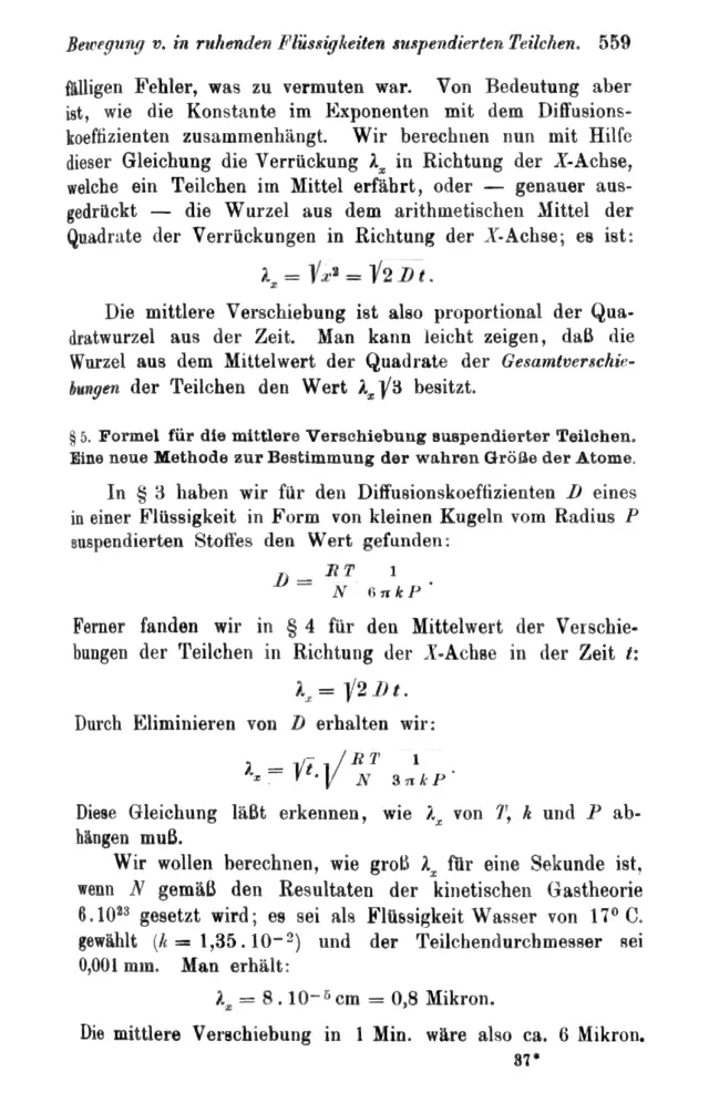
The 3 printed paragraphs this passage explains

§5, paragraph 2: Taking N as 6 · 10²³ from the kinetic theory of gases, water at 17 °C as the liquid, and particles 0.001 mm across, λx for one second comes to 8 · 10⁻⁵ cm, or 0.8 micron, and about 6 microns in one minute.
§5, paragraph 3: Turned around, the same relation can be used to determine N from observed displacements.
§5, paragraph 4: Einstein closes by hoping that a researcher will soon succeed in deciding the question raised here, which he calls important for the theory of heat.

D = \frac{\left\langle x^{2}\right\rangle}{2\,t}

N = \frac{R\,T\,t}{3\,\pi\,\eta\,a\,\left\langle x^{2}\right\rangle}

Shown in modern letters; Einstein's are in §5 of the German source face.

Diffusivity is the mean-square displacement divided by twice the time; the molecular number is the gas constant times temperature times time, divided by three pi times viscosity times radius times the mean-square displacement.

The first expression refers to the model mean square, or to an estimate obtained from an appropriate sample. The second is an inversion under the stated physical assumptions. An estimate needs uncertainty and checks of those assumptions; rearranging symbols does not remove experimental error.

Without an independent radius, the same D can result from many pairs of a and N. The data then select a compatible family rather than a unique molecular number. The existing synthetic laboratories explore this relationship but do not supply a historical measurement.

Open the foundation: Two measurements, two unknowns

Open the foundation: Mean, variance and RMS

Open the foundation: Uncertainty, evidence and inference

Open the foundation: The units of 1905

Show every step here: What would let us count molecules?

Start from the displacement law of §4, $\langle x^2\rangle = 2Dt$ . Here $\langle x^2\rangle$ is the mean-square displacement along one axis after an observation time $t$ , and $D$ is the tracers’ diffusivity. Divide both sides by $2t$ , which is allowed for any positive $t$ : $D = \langle x^2\rangle/(2t)$ .
Next, the physical relation of the previous passage, $D = RT/(6\pi\eta aN)$ , where $R$ is the gas constant, $T$ the absolute temperature, $\eta$ the viscosity (Einstein’s $k$ ), $a$ the tracer radius (his $P$ ) and $N$ the number of molecules in a mole.
Solve it for $N$ . Multiply both sides by $6\pi\eta aN$ , giving $6\pi\eta aND = RT$ . Then divide both sides by $6\pi\eta aD$ : $N = RT/(6\pi\eta aD)$ .
Put the first result in for $D$ . Dividing by a fraction is multiplying by its inverse, so dividing by $\langle x^2\rangle/(2t)$ multiplies by $2t/\langle x^2\rangle$ : $N = RT \cdot 2t/(6\pi\eta a\langle x^2\rangle)$ .
The 2 above and the 6 below leave a 3 below, since 2/6 = 1/3. Einstein prints this inversion at the end of §5 as $N = \frac{t}{\lambda_x^2}\cdot\frac{RT}{3\pi kP}$ , with $\lambda_x^2$ for the mean square, his $k$ for $\eta$ and his $P$ for $a$ . The two results together:

D = \frac{\left\langle x^{2}\right\rangle}{2\,t}

N = \frac{R\,T\,t}{3\,\pi\,\eta\,a\,\left\langle x^{2}\right\rangle}

Shown in modern letters; Einstein's are in §5 of the German source face.

Read what each symbol needs. In the formula $\langle x^2\rangle$ is the model’s mean square. From a finite set of tracked particles you get an estimate of it, and that estimate has an uncertainty the formula does not show. Rearranging the symbols carries that uncertainty into $N$ ; it does not remove it.
$R$ , $T$ , $\eta$ and $a$ must each be measured separately, and all in one system of units. The inversion also holds only under the assumptions that gave $D = RT/(6\pi\eta aN)$ : few, small spheres in a liquid, Stokes’s drag and ideal osmotic pressure. An estimate needs checks of those assumptions as well as its uncertainty.
The radius matters most. In $D = RT/(6\pi\eta aN)$ , $a$ and $N$ appear only as the product $aN$ . A measured $D$ fixes that product, $aN = RT/(6\pi\eta D)$ , and nothing more: halve $a$ and double $N$ , and $D$ is unchanged. Without an independent radius, the data select a family of compatible pairs rather than one molecular number.
Run Einstein’s §5 case through the formulas. His inputs are $T$ = 290.15 K (water at 17 °C), $\eta$ = $1.35\times10^{-3}$ Pa·s, $a$ = $5\times10^{-7}$ m and $N$ = $6\times10^{23}$ , with $R$ = 8.31 J/(mol·K) supplied by this edition. The previous passage found $D$ = $3.16\times10^{-13}$ $\mathrm{m}^2/\mathrm{s}$ from them, so at $t$ = 1 s the mean square is $6.32\times10^{-13}$ $\mathrm{m}^2$ , an RMS of 0.795 μm.
Now invert. $RTt$ = 8.31 × 290.15 × 1 = 2411 J·s/mol. $3\pi\eta a\langle x^2\rangle$ = 3π × ( $1.35\times10^{-3}$ ) × ( $5\times10^{-7}$ ) × ( $6.32\times10^{-13}$ ) = $4.02\times10^{-21}$ J·s. Their quotient is $N$ = $6.0\times10^{23}$ per mole: the $N$ that went in.
That checks the arithmetic of the inversion and nothing else. It cannot count molecules, because the mean square fed into it was computed from an assumed $N$ . In §5 Einstein ran the relation forward in this way, as a prediction, and printed the inversion for a future measurement to use; he did not estimate $N$ himself.
The same numbers show the family. With this $D$ , the product $aN$ is $3.0\times10^{17}$ metres per mole. A radius of 0.5 μm gives $N$ = $6\times10^{23}$ ; had the radius been 1 μm, the same $D$ would give $N$ = $3\times10^{23}$ . Only an independent measurement of $a$ chooses between them.
A simulation that uses an assumed molecular number can test this inversion’s arithmetic in the same way, but cannot independently establish that number in nature.

A tool for this step

Two measurements, two unknowns

Can a measured spreading rate tell you how big the particle is?

In §5 of the Brownian paper the diffusion coefficient of a suspended sphere is $D = \frac{RT}{N}\cdot\frac{1}{6\pi\eta a}$ . Einstein writes k for the viscosity and P for the radius; this lesson uses η and a. At a fixed temperature and viscosity, a measured D fixes one combination of the two unknowns, the product of the molecular number N and the radius a.

N\,a = \frac{R\,T}{6\,\pi\,\eta\,D}

N times a equals R T divided by six pi eta D.

Every pair with that product fits the measurement equally well. Drawn in a plane with the radius along one axis and the molecular number along the other, the pairs form a curve. Double the radius and halve N, and the product, and with it D, is exactly what it was. Displacements alone cannot say which point on the curve is the true one, and measuring D more carefully does not change that.

Einstein's dissertation measured something else: how much a dissolved substance thickens water. The volume taken up by the dissolved particles, as a fraction of the whole, is $\varphi = \frac{4}{3}\pi a^3 N n$ , where n is the number of moles dissolved per unit volume. The viscosity relation therefore fixes a different combination, $a^3 N$ . Its curve in the same plane has another shape, and the two curves cross.

a^{3}\,N = \frac{3\,\left(\frac{\eta^*}{\eta} - 1\right)}{4\,\pi\,c\,n}

a cubed times N equals three times the quantity eta star over eta minus one, divided by four pi c n.

Here $\eta^*$ is the viscosity of the solution, η that of the water, and c the coefficient of φ in the viscosity law: 1 as the dissertation printed it in 1906, and 5/2 after Einstein's correction of 1911. This lesson takes the relation as given: deriving it, and the history of its correction, belong to the dissertation. Dividing the second combination by the first leaves $a^2$ alone, so the crossing gives the radius, and then either relation gives N.

a^{2} = \frac{3\,\left(\frac{\eta^*}{\eta} - 1\right)}{4\,\pi\,c\,n}\,\frac{6\,\pi\,\eta\,D}{R\,T}

a squared equals three times the quantity eta star over eta minus one, over four pi c n, times six pi eta D over R T.

A crossing is not yet an answer. Two curves that cross at a shallow angle fix their crossing poorly, so a small error in either measurement moves it a long way. Each measurement has an uncertainty, which widens its curve into a band, and the honest result is the region where the two bands overlap, not a point. Two measurements that rest on the same calibration can cross and still add nothing new. And each relation holds only within its own domain: dilute suspensions, spheres much larger than the molecules of the liquid.

Worked example: Why solving for the radius gives a curve

The question: can a measured spreading rate tell you how big the particle is?
What is given: the measured D, the temperature T, the viscosity η, and the relation $D = RT/(6\pi\eta a N)$ .
The first thought, and a reasonable one: solve the relation for a. The algebra looks as if it allows that.
The decisive step: solving gives $a = RT/(6\pi\eta N D)$ , the radius in terms of N. Every choice of N gives its own a. Double a and halve N, and $6\pi\eta a N$ , and with it D, is exactly what it was. The answer is a curve, not a number.
The limitation: a second relation that depends on a and N in another way is needed. How well it fixes the pair depends on the angle at which the two curves cross and on the two measurements being independent, and what comes out is a region, not a point.

JavaScript is off, so the controls below cannot change anything. The construction shows its first setting, and its closing paragraph, “What it shows, in words”, describes the rest.

Try it: where two measurements cross

The plane holds every pair of a radius and a molecular number, each drawn as a multiple of the true value, on scales where equal steps mean equal factors. Diffusion fixes N·a, a band of slope −1. A second measurement that fixes a^k·N is a band of slope −k; the viscosity measurement of the dissertation has k = 3. Both are drawn centred on the true pair, as if each measurement had landed on it, and as wide as its stated spread.

How steep the second band is

How wide each band is

The radius lies between 0.95 and 1.05 times the true radius, and N between 0.90 and 1.11 times the true N. That is the overlap of the two stated spreads, not a probability.

The dissertation's own inversion, from a measured diffusion coefficient and a solution's viscosity, runs in the molecular-dimensions companion preview, with the viscosity coefficient as printed in 1906 or as corrected in 1911.

What it shows, in words

With diffusion alone, the pairs that fit form a band running the whole width of the plane: a smaller radius with a larger N fits exactly as well. A second measurement of a different combination is a band at a different slope, and the two cross in a small region around the true pair. The more the slopes differ, the smaller that region: at k = 3 and a spread of 5 per cent on each, the radius is fixed to within about 5 per cent. As k comes down towards 1 the bands turn parallel and the region stretches along them, because a small error in either measurement moves the crossing a long way. At k = 1 both measurements fix the same product and the radius is not fixed at all.

Where this lesson stops

One measurement of one combination of two quantities leaves a curve, not a point.

A tool for this step

Mean, variance and RMS

If particles wander both ways, which average shows how far they got?

Four particles move −3, −1, +1 and +3 micrometres. Their average position has not changed, yet they have spread out. Three averages answer three different questions.

\left\langle x\right\rangle = \frac{1}{M}\,\sum_{i=1}^{M} x_{i}

Add the M signed displacements and divide by M.

\left\langle x^{2}\right\rangle = \frac{1}{M}\,\sum_{i=1}^{M} x_{i}^{2}

Square each displacement before adding and dividing by M.

\operatorname{Var}\left(x\right) = \left\langle x^{2}\right\rangle - \left\langle x\right\rangle^{2}

Variance is the mean square minus the square of the mean.

RMS means root mean square: average the squares, then take the square root. The standard deviation is the square root of the variance, so it measures spread around the mean, where the RMS measures distance from zero. The two are equal only when the mean is zero. The average of the distances, ignoring sign, is a third statistic and gives a different number.

Worked example: Four displacements, four different averages

For −3, −1, +1, +3 the signed sum is 0, so the mean is 0.
The distances, ignoring sign, are 3, 1, 1, 3; their mean is 2.
The squares are 9, 1, 1, 9; their mean is 5.
The RMS is the square root of 5, about 2.236. With a mean of 0, the variance is also 5 and the standard deviation is also about 2.236.
A small random sample need not have a signed mean of exactly zero, even when the model's mean is zero.

One question, three answers

The four displacements the lesson counts, on a ruler through the start. Two went left and two went right, by matching amounts.

Now the three averages on one scale of distance from the start. They are three different numbers because they answer three different questions.

The mean square, 5 square micrometres, is not on that scale and could not be: it is an area. Taking its square root is what brings it back to a distance, and that root, about 2.236, sits a little beyond the average distance of 2.

What it shows, in words

The first drawing puts the four displacements, -3, -1, 1, 3 micrometres, on a ruler through the start. Two are left of zero and two right of it at matching distances, so the average position is 0: the particles have spread out and their average has not moved at all.

The second puts three averages on one scale of distance. The average position is 0. The average of the distances, ignoring sign, is 2. The root mean square is about 2.236, a little farther out, because squaring weighs the two particles that went three micrometres more heavily than the two that went one. The mean square, 5 square micrometres, is not drawn there: it is an area, and putting it beside two lengths would be the mistake the lesson exists to prevent.

What it does not show: these four are one sample, not the model behind it. A small random sample need not have a signed average of exactly zero even when the model's is zero, and nothing in either drawing distinguishes a real cancellation from a lucky one. The root mean square and the standard deviation are the same number here only because this average happens to be zero; where it is not, they part company, and neither drawing shows that.

Where this lesson stops

Say which average you mean. Squaring then averaging, averaging then squaring, and averaging the distances give three different numbers.

Going further: One sample's mean square, and what the microscope adds

In the Brownian problem the model's mean square displacement along one coordinate is 2Dt. A sample's mean square is an estimate of it: average the squares of the displacements actually measured, then divide by 2t to estimate D. If the four displacements above, −3, −1, +1 and +3 μm, were measured after t = 1 s along one coordinate, their mean square of 5 μm² would give D = 5 ÷ 2 = 2.5 μm² per second.

Averaged over many samples, this estimate lands on the true value: it has no bias. One sample scatters, and the scatter shrinks only with the square root of the number q of independent squared displacements. For displacements drawn from the bell curve, the spread of the estimate, as a fraction of the true value, is:

\frac{\mathrm{spread}}{D}=\sqrt{\frac{2}{q}}

The spread of the estimate, divided by D, equals the square root of two over q.

With q = 4, as above, the spread is about 71 per cent of D, so four particles say little.
With q = 100 it is about 14 per cent.
To halve the spread, measure four times as many independent displacements.

If the particles might also drift, the mean has to be estimated from the same numbers. The average squared deviation from that estimated mean then comes out too small, by the factor (M − 1)/M on average, because the estimated mean sits closer to the sample than the true one does. Dividing the sum by M − 1 instead of M removes that bias.

The microscope adds an error of its own. A measured step is the difference of two position readings, so if each reading is off by an error of spread σ in each coordinate, the step's mean square gains 2σ² per coordinate. For D = 0.5 μm² per second and t = 1 s the true mean square is 2Dt = 1 μm². A reading error of σ = 0.1 μm adds 0.02 μm², 2 per cent; σ = 0.3 μm adds 0.18 μm², 18 per cent. Unless it is subtracted, all of it is read as extra diffusion.

Two neighbouring steps share the reading between them, so their errors are related, with a covariance of −σ². The steps are then not independent, and cutting one path into overlapping windows does not help: the windows reuse the same readings, so they do not add independent squares to q.

Open the foundation: Uncertainty, evidence and inference

A tool for this step

Uncertainty, evidence and inference

What can a set of measurements tell you, and what can it not?

Some questions the data cannot answer, however carefully you measure. If all you know of a rectangle is that its area is 12 square centimetres, its sides could be 3 and 4, 2 and 6, or 1 and 12. The area fixes their product, not each side; to get one side you must measure the other.

The Brownian paper meets the same limit. In its §3 the diffusion coefficient is D = RT/(N · 6πkP), with k the liquid's viscosity and P the particle's radius. So watching particles spread gives D, and with the temperature and viscosity known, D fixes the product of N and P, not each of them: a smaller particle and a larger N give the same spreading. To get N, the radius has to be measured some other way.

An estimate comes from a finite sample, and a different sample gives a different number. Two questions follow: whether the method lands on the right value on average, which is its bias, and how widely its answers scatter from sample to sample. Fitting a drift from the same displacements uses up part of the information and leaves less to estimate the scatter.

Uncertainty comes in four kinds, and each needs its own statement. Sampling uncertainty is the scatter from one sample to the next. Measurement uncertainty is the error in each reading, such as where the microscope places a particle. Model uncertainty is the chance that the formula itself does not fit these particles. Numerical uncertainty is the error of the computation. A confidence interval is not an interval-arithmetic enclosure, which is guaranteed to contain the exact result of a calculation, and a numerical error bar, which bounds the arithmetic, is not a measurement uncertainty.

A 95 per cent confidence interval comes from a method that, used on many samples, catches the true value in 95 of every 100 of them, provided its assumptions hold. It is not a 95 per cent chance that this one interval contains the value. A plot of many repeated intervals, with the misses left in, shows what the promise means.

For a diffusion coefficient the promise has an exact form. With M independent displacements in d coordinates there are q = dM squared displacements, and their sum divided by 2Dt has a known spread from sample to sample: the chi-square distribution with q degrees of freedom. Its 2.5 and 97.5 per cent points give the 95 per cent interval. In a synthetic example with 50 displacements in two coordinates, so q = 100, and an estimate of 0.43 μm²/s, those points are 74.2219 and 129.5612:

\begin{aligned} &\left[\frac{100 \times 0.43}{129.5612},\ \frac{100 \times 0.43}{74.2219}\right] \\ &\quad = [0.3319,\ 0.5793]\ \mu\mathrm{m}^2/\mathrm{s} \end{aligned}

The interval runs from 43 divided by 129.5612 to 43 divided by 74.2219, that is from 0.3319 to 0.5793 square micrometres per second.

Inverting an estimate adds a bias of its own. The molecular number is found by dividing by the estimated D, and although that estimate is right on average, its reciprocal is not: with q = 100 degrees of freedom the average of the inverted estimate is too large by the factor q/(q − 2) = 1.020408, about two per cent. The interval itself survives inversion, with its ends swapped, as the worked example shows.

Reading positions adds noise of its own. If each position is read with an error of spread σ in each coordinate, each measured step gains 2σ² in its mean square per coordinate, and two neighbouring steps share one reading, so their errors have a covariance of −σ². Neighbouring steps are then no longer independent, and cutting one path into overlapping windows does not make independent samples.

An interval that treats the radius, viscosity and temperature as exact holds only on that condition. Allowing for their uncertainty needs to know how each was measured and how often its own interval misses. Without that, a plus-or-minus has no stated coverage and is not a confidence statement.

A path simulated from a chosen N is useful for checking that a method recovers the N it was given. It is not evidence about N in nature. Since 2019 the SI fixes Avogadro's number by definition, so recovering it from modern data checks consistency. Measuring N, as Perrin did from 1908, needs inputs measured independently of it.

Worked example: Inverting an interval, and watching its endpoints swap

Take a made-up relation, N = 12/D, with D measured as 4. The estimate is N = 12/4 = 3.
Suppose the method gives D between 3 and 6. A larger D means a smaller N, so N runs from 12/6 = 2 to 12/3 = 4: the ends swap over.
Now suppose N = 12/(aD), with a an unknown scale. The same D fits many pairs of a and N, and no interval for N follows until a is measured separately.
Declaring a = 2 halves both the estimate and its interval without changing a single measurement. It changes an assumption, not the data.
If three inputs each come from a method that misses at most once in 100 uses, and D's method at most twice, the combination misses at most 5 times in 100, even if the misses are related. Without the stated miss rates, this arithmetic guarantees nothing.

JavaScript is off, so the controls below cannot change anything. The construction shows its first setting, and its closing paragraph, “What it shows, in words”, describes the rest.

One area, three shapes

Every rectangle below encloses 12 square centimetres. They are drawn at one scale, so the areas really are equal and the shapes really are not.

The measurement fixes the product and leaves the pair open. That is not a shortcoming of the measuring: no amount of care with the area will separate 3 and 4 from 1 and 12. Another kind of observation has to do it.

What it shows, in words

Three rectangles at one scale, each enclosing 12 square centimetres: 3 by 4, 2 by 6, 1 by 12. The first is nearly square, the last is a thin sliver twelve centimetres tall, and no measurement of area however careful will tell you which one you have. The area fixes the product of the sides and says nothing about either side alone.

The Brownian paper meets the same limit in its §3. Watching particles spread gives the diffusion coefficient, and the diffusion coefficient fixes a product of the molecular number and the particle radius. One more independent measurement, of the radius, is what separates them, exactly as a second measurement of one side would separate these rectangles.

What it does not show: three is not the family. Any pair whose product is 12 lies on the same curve, including pairs that are not whole numbers, such as 2.5 by 4.8. These three are drawn because they are the three the lesson names, not because the possibilities can be counted, and a reader who took the picture for the whole set would be reading a limit into it that is not there.

Try it: many experiments, many intervals

A made-up generator produces particle paths with a diffusion coefficient of 0.43 μm²/s. Each experiment estimates it from q squared displacements and forms the 95 per cent interval. Count how many of the intervals catch the value the generator used.

19 of 20 intervals cover 0.43 μm²/s. The procedure promises 95 of every 100 in the long run; a set of 20 can land a little above or below that.

Seed 1906, q = 100.

All 20 experiments

Each line runs from 0 at the left to 1 μm²/s at the right. The upright mark is 0.43, the value the generator used.

Experiment 1: 0.371 to 0.648 μm²/s, covers
Experiment 2: 0.349 to 0.610 μm²/s, covers
Experiment 3: 0.350 to 0.612 μm²/s, covers
Experiment 4: 0.325 to 0.568 μm²/s, covers
Experiment 5: 0.356 to 0.622 μm²/s, covers
Experiment 6: 0.337 to 0.588 μm²/s, covers
Experiment 7: 0.343 to 0.599 μm²/s, covers
Experiment 8: 0.381 to 0.665 μm²/s, covers
Experiment 9: 0.329 to 0.574 μm²/s, covers
Experiment 10: 0.285 to 0.498 μm²/s, covers
Experiment 11: 0.347 to 0.606 μm²/s, covers
Experiment 12: 0.377 to 0.659 μm²/s, covers
Experiment 13: 0.321 to 0.560 μm²/s, covers
Experiment 14: 0.346 to 0.603 μm²/s, covers
Experiment 15: 0.325 to 0.567 μm²/s, covers
Experiment 16: 0.321 to 0.560 μm²/s, covers
Experiment 17: 0.297 to 0.518 μm²/s, covers
Experiment 18: 0.343 to 0.599 μm²/s, covers
Experiment 19: 0.201 to 0.352 μm²/s, misses
Experiment 20: 0.312 to 0.545 μm²/s, covers

What it shows, in words

Every experiment gives a different interval, because every sample is different. The value the generator used never moves; the intervals move around it. Over many experiments about 95 in 100 intervals cover it and the rest miss, which is all the 95 per cent promises. With q = 10 the intervals are much wider than with q = 100, and the promise is the same. The data here are made up, so the view tests the procedure, not molecules.

Where this lesson stops

Say what the data can tell apart, which method and model you used, what you held exact, and whether the result recovers a value you put in, estimates it independently, or checks consistency.

A tool for this step

The units of 1905

How do Einstein's numbers, printed in centimetres, grams, ergs and the old electrical units, become SI units?

Einstein's papers measure length in centimetres, mass in grams and time in seconds, the CGS system. Energy is in ergs, and one erg is 10⁻⁷ joules. Viscosity is in grams per centimetre per second, the unit now called the poise, and one poise is 0.1 pascal-seconds. These mechanical factors are exact, because they follow from 1 cm = 0.01 m and 1 g = 0.001 kg.

To convert, multiply by a ratio equal to one. Since 1 poise is 0.1 pascal-seconds, the ratio (0.1 Pa s)/(1 P) equals one, and multiplying by it changes the unit without changing the viscosity. The Brownian paper gives water's viscosity as 1,35 · 10⁻², with no unit name; it is in poise, so the viscosity is 1.35 × 10⁻³ Pa s. The paper calls this viscosity k, which is not Boltzmann's constant.

\begin{aligned} &1.35\times10^{-2}\,\mathrm{P}\times\frac{0.1\,\mathrm{Pa\,s}}{1\,\mathrm{P}} \\ &\quad = 1.35\times10^{-3}\,\mathrm{Pa\,s} \end{aligned}

1.35 times ten to the minus two poise, times 0.1 pascal-seconds per poise, equals 1.35 times ten to the minus three pascal-seconds.

The same ratio works for compound units. The gas constant R = 8.31 × 10⁷ erg per mole per kelvin is 8.31 joules per mole per kelvin. Neither the light paper nor the Brownian paper prints this number; the edition supplies the standard value of 1905 as an editorial input and labels it that way.

Electricity had two CGS systems. The electrostatic system builds its charge unit, the statcoulomb, from the force between charges. The electromagnetic system builds its current unit from the force between currents; its units are the abcoulomb and the abvolt. One abcoulomb is 10 coulombs, one abvolt is 10⁻⁸ volts, one statvolt is 299.792458 volts, and one gauss is 10⁻⁴ tesla. Planck's 1901 elementary charge, 4,69 · 10⁻¹⁰ statcoulombs, is 1.56 × 10⁻¹⁹ coulombs.

These electrical correspondences are conventional, not exact. They assume the magnetic constant $\mu_0$ is exactly 4π × 10⁻⁷ henry per metre. Since the 2019 revision of the SI it is a measured quantity, equal to that value within about one part in a billion. The site marks every electrical conversion conventional.

The light paper's photoelectric check in §8 uses the electromagnetic system. It takes E = 9,6 · 10³ for the charge of one gram-equivalent of a monovalent ion, so a potential Π comes out in abvolts, and the paper multiplies by 10⁻⁸ to get volts. It prints the result as about 4,3 volts. On the result line the factor is set as 10⁷; the edition records this as a misprint, because the sentence four lines earlier gives 10⁻⁸. The check can also be run per electron, with Planck's charge in statcoulombs and the result in statvolts, and it gives 4.31 volts; the edition keeps that as a documented alternative and follows the page.

The paper's R, E and J are amounts per gram-equivalent, a mole of monovalent ions. Dividing by N gives the amount per molecule, R/N, or per electron, ε. With the paper's E and the N it prints in §2, 6,17 · 10²³, the charge on one ion is 9.6 × 10³ ÷ 6.17 × 10²³ = 1.56 × 10⁻²⁰ abcoulombs, which is 1.56 × 10⁻¹⁹ coulombs. The paper does not print this quotient.

The relativity paper writes its fields in Gaussian units, where electric and magnetic fields share one unit. That is why its transformation reads β(Y − (v/V)N), with the dimensionless ratio v/V; here N is a magnetic field component, not Avogadro's number. SI measures the electric field in volts per metre and the magnetic field in tesla, so the same law reads $\gamma(E_y - vB_z)$ , with the speed itself multiplying the magnetic field. One statvolt per centimetre is 2.998 × 10⁴ volts per metre.

\begin{gathered} 1\,\mathrm{abV} = 10^{-8}\,\mathrm{V}, \\ 1\,\mathrm{abC} = 10\,\mathrm{C}, \\ 1\,\mathrm{statV} = 299.792458\,\mathrm{V}, \\ 1\,\mathrm{G} = 10^{-4}\,\mathrm{T} \end{gathered}

One abvolt corresponds to ten to the minus eight volts, one abcoulomb to ten coulombs, one statvolt to 299.792458 volts, and one gauss to ten to the minus four tesla, all by convention.

Worked example: The photoelectric check, converted to volts

The inputs: β = 4,866 · 10⁻¹¹ and ν = 1,03 · 10¹⁵ per second are printed in §8, and so is E = 9,6 · 10³. R = 8.31 × 10⁷ erg per mole per kelvin is the edition's editorial input, because the paper does not print it.
With P′ = 0, Π = Rβν/E = 8.31 × 10⁷ × 4.866 × 10⁻¹¹ × 1.03 × 10¹⁵ ÷ 9.6 × 10³ = 4.34 × 10⁸ abvolts.
Multiply by the ratio 10⁻⁸ volts per abvolt: 4.34 volts. The paper prints about 4,3 volts.
In §9 the conversion runs the other way. An energy per gram-equivalent divided by E is a potential: the printed Rβν = 6,4 · 10¹² erg gives 6.4 × 10¹² ÷ 9.6 × 10³ = 6.67 × 10⁸ abvolts, or 6.67 volts.
Stark's ionization voltage of 10 volts is 10⁹ abvolts, and 10⁹ × 9.6 × 10³ = 9.6 × 10¹² erg per gram-equivalent, the upper bound for J that §9 prints.
E itself, 9.6 × 10³ abcoulombs, is 9.6 × 10⁴ coulombs per gram-equivalent. Beside it, the modern Faraday constant is 96 485 coulombs per mole (set modern-si-2019); Einstein's value is 0.50 percent below it.

JavaScript is off, so the controls below cannot change anything. The construction shows its first setting, and its closing paragraph, “What it shows, in words”, describes the rest.

Try it: converting a printed number

Type a number and choose the unit it was printed in. The calculator multiplies by a ratio equal to one, taken from the site's table of units, and says whether that ratio is exact or a convention.

Number to convert

Write 1.35e-2 or 1,35 · 10^-2. A comma is read as a decimal comma, as the papers print it.

Its unit, and the SI unit to convert to

0.0135 P = 0.00135 Pa s

Ratio used: 1 P = 0.1 Pa s.

Exact: it follows from 1 cm = 0.01 m and 1 g = 0.001 kg.

The papers' own numbers, converted

Water's viscosity, which the paper calls k (Brownian motion, p. 559): 0.0135 P = 0.00135 Pa s. Exact.
The gas constant R (not printed in either paper; supplied by the edition): 8.31 × 10⁷ erg per mole per kelvin = 8.31 J per mole per kelvin. Exact.
E, the charge of one gram-equivalent of a monovalent ion (Light quanta §8, p. 146): 9.6 × 10³ abC per gram-equivalent = 9.6 × 10⁴ C per gram-equivalent. Conventional.
Π = Rβν/E with P′ = 0; the paper prints only the result, about 4,3 volts (Light quanta §8, computed in the worked example): 4.34 × 10⁸ abV = 4.34 V. Conventional.
Rβν for the longest effective wavelength in air (Light quanta §9, p. 148): 6.4 × 10¹² erg per gram-equivalent = 6.4 × 10⁵ J per gram-equivalent. Exact.
The elementary charge (Planck 1901, p. 565): 4.69 × 10⁻¹⁰ statC = 1.56 × 10⁻¹⁹ C. Conventional.

What it shows, in words

A number printed in a CGS unit becomes an SI number when it is multiplied by a ratio equal to one. The mechanical ratios are exact. The electrical ratios are conventional, because they take the magnetic constant as exactly 4π × 10⁻⁷ H/m. The calculator converts units only: it never replaces a historical constant with a modern one.

Where this lesson stops

A conversion factor is a ratio equal to one. This lesson converts units only: it never turns a historical constant's value into a modern one, and it treats every electrical correspondence as a convention.

Explore the equations in this step

Read each operation, check its units and assumptions, or open the mathematical step behind it. These are modern teaching equations, not the equations as printed.

Explore the equation · Modern model notation

From a measured spread to the number of molecules

N = \frac{R\,T\,t}{3\,\pi\,\eta\,a\,\left\langle x^{2}\right\rangle}

Shown in modern letters; Einstein's are in §5 of the German source face.

is times times over three pi times , and the mean of squared.

Select a term or operation. In the formula, Down enters an operation, Up returns to its parent, and Left/Right move between siblings. Escape clears selection. Tab leaves the formula.

Explain this equation

Each term and operation, in words

No live values

This equation states a relation. No instrument on this page computes its terms.

Read the equation aloud in words

Avogadro's number N equals the gas constant times the temperature times the observation time, divided by the product of three pi, the viscosity, the particle radius and the mean square displacement.

With temperature, viscosity and radius measured independently, the observed mean square gives Avogadro's number. The radius has to come from somewhere else: the spread alone cannot separate it from N.

Model assumptions and every term’s meaning

Radius, viscosity and temperature are measured independently of the displacement data.
The same dilute-sphere model as the diffusivity.
These are modern teaching equations in SI notation, not a transcription of the printed paper. The paper writes k for the viscosity.

Three pi eta a times the mean square: Drag and the observed spread. Read the prerequisite
The observed mean square: From many displacements. Read the prerequisite
R T t: Thermal energy per mole, times the interval. Read the prerequisite
The ratio: Per mole. Read the prerequisite
What it asserts: Counting molecules becomes a measurement of spreading. Read the prerequisite
x squared: Each observed displacement, squared. Read the prerequisite
Displacement since the start: How far one particle has moved along x since observation began. Read the prerequisite
Estimated Avogadro number: The number of molecules per mole this measurement infers. An estimate, not the defined constant. Read the prerequisite
Gas constant: Energy per mole per kelvin. Read the prerequisite
Particle radius: The radius of the suspended sphere, not its diameter. Read the prerequisite
Absolute temperature: Temperature in kelvin. Read the prerequisite
Observation interval: The time over which displacement is observed. Read the prerequisite
Viscosity: The liquid's resistance to shear. The paper writes it k, which is not Boltzmann's constant. Read the prerequisite

Every term’s units were checked when this page was built. That checks the units, not the model. This equation is written for this edition in modern notation, not transcribed from the paper.

Explore the equation · Modern model notation

Read D off the observations

D = \frac{\left\langle x^{2}\right\rangle}{2\,t}

Shown in modern letters; Einstein's are in §5 of the German source face.

is the mean of squared over two .

Select a term or operation. In the formula, Down enters an operation, Up returns to its parent, and Left/Right move between siblings. Escape clears selection. Tab leaves the formula.

Explain this equation

Each term and operation, in words

No live values

This equation states a relation. No instrument on this page computes its terms.

Read the equation aloud in words

D equals the mean square displacement over two t.

Turn the relation around: a measured mean square over a known interval gives D.

Model assumptions and every term’s meaning

The mean square is estimated from many observed displacements over one interval t.
These are modern teaching equations in SI notation, not a transcription of the printed paper.

Two t: Twice the interval. Read the prerequisite
Their mean: An estimate from a finite sample. Read the prerequisite
Mean square over two t: Metres squared per second. Read the prerequisite
What it asserts: D is measurable from displacements alone. Read the prerequisite
x squared: Each observed displacement, squared. Read the prerequisite
Diffusion coefficient: How fast the mean square displacement grows: half its rate of growth. Not a speed. Read the prerequisite
Displacement since the start: How far one particle has moved along x since observation began. Read the prerequisite
Observation interval: The time over which displacement is observed. Read the prerequisite

Every term’s units were checked when this page was built. That checks the units, not the model. This equation is written for this edition in modern notation, not transcribed from the paper.

Modern qualifications

Einstein did not estimate $N$ . He took $N = 6 \times 10^{23}$ from the kinetic theory of gases and predicted a displacement of about 0.8 μm in one second for particles 0.001 mm across in water at 17 °C, closing with the hope that someone would soon test it. Jean Perrin’s measurements from 1908 onward did, and gave values of $N$ near $7 \times 10^{23}$ . This page supplies no dataset of its own.

Assumptions and limits: What would let us count molecules?

Assumed here

A measured mean-square displacement along one axis, or how fast it grows with time.
Separately measured R, T, η and particle radius a, for few small spheres in a liquid.

What this does not establish

A synthetic run generated from an assumed N is not independent evidence for N.
Without the radius, the diffusivity fixes only the product aN.
Measurement noise, drift, exposure and finite sampling require separate treatment.

Earlier step: Why viscosity changes the spread

Source context: Annalen der Physik (4), 17, 549–560 (1905), §§1–5. Bibliographic pointer; this preview is not a source transcription or translation.

Explanation

Einstein's displacement argument: the typical distance grows with the square root of time, not with time itself. Every explanation stays on the page when reading-only is on.

Static worked case

For radius 0.5 μm, viscosity 1.35×10⁻³ Pa·s, and T = 290.15 K, the RMS displacement is about 0.8 μm in one second. This static worked case stays in the markup; loading the live ensemble does not replace it.

Try the displacement argument yourself

Once open, the tracer ensemble stays open while you change the detail or read a lesson. It runs a new trial only when you apply its settings; opening an explanation never starts one.

Open the tracer ensemble in this reading

Open the tracer ensemble on its own page, where its worked example is part of the page.

Notes and laboratory

Page 559 of Annalen der Physik, volume 17, where §5 begins. — §5 begins on page 559 of Annalen der Physik, volume 17. Read it in Einstein’s German

Symbols in §5

Estimated Avogadro number
Gas constant
Absolute temperature
Observation interval
Dynamic viscosity
Particle radius
Displacement since the start
Diffusion coefficient

Keep the tracer ensemble in view

Read in another form

Download the full explanation as Markdown · The same explanation as data (JSON) · Browse the foundation library

Read this offline

Each chapter is one HTML file that opens in any browser without a connection. It holds the explanation at every level of detail, the lessons it links to, its source references and the numbers worked out when the site was built. It has no notes of yours and no running simulations. It is an explanation, not an edition of the paper.

Download §5 · From displacement to molecular scale HTML, 651 KB

Links to online sources still need a connection, and the interactive plots are not included. Every chapter you can keep

Original journal scan